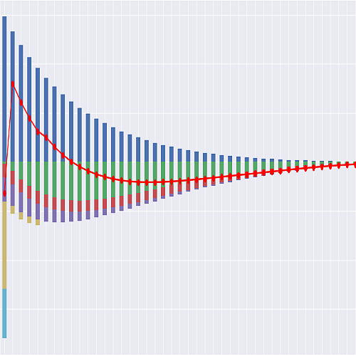
Validation#
Checks of the G2PP space against closed forms and martingale properties.
Every test returns a DataFrame with the columns
mc: the Monte Carlo estimate over the stochastic scenarios 1 to N,theory: the value it should converge to,se: its standard error, from antithetic pair means when antithetic variates are on,z: \((\mathrm{mc} - \mathrm{theory}) / \mathrm{se}\).
With correct formulas, each z is roughly standard normal, so \(|z| > 3\) is rare for a
single check. Tests that cover many months or moments contain many z-scores, so a larger
maximum is expected by chance: summary() compares the largest \(|z|\) of each
test with a limit that allows for the number of z-scores. Where the estimate is exact by
construction, z is 0 (see mcstats.check).
The tests read the scenarios through the Reference g2pp, so they run on whatever
input the G2PP space uses. Statistical power grows with scen_size; 10,000 antithetic
scenarios is a good setting for validation.
- g2pp#
The G2PP space.
- mcstats#
User module with
check(), which turns samples into the DataFrame above. Saved in the model folder asmcstats.py.
- np#
The numpy module.
- pd#
The pandas module.
- stats#
The scipy.stats module, for the normal distribution.
Cells
Spot rates implied by the mean deflators against the input curve |
|
|
Call on the deflator \(D(t_i)\) with strike \(K = k P^M(0, t_i)\) |
Deflated value of the selected fund against 1, for every month |
|
Mean deflator against the initial curve, for every month |
|
Means, variances and covariance of \(x\), \(y\) and \(r\), every year |
|
|
Largest \(|z|\) of each test on the current input, against its limit |
|
Closed-form price of a put on a zero-coupon bond (Brigo and Mercurio, section 4.2) |
|
Monte Carlo price of the bond put of |
|
Deflated bond prices: \(E[D(t_i) P(t_i, t_j)] = P^M(0, t_j)\) |
- martingale_test()[source]#
Mean deflator against the initial curve, for every month
\(E[D(t_i)] = P^M(0, t_i)\) for i = 0 to n.
- Returns:
pandas.DataFrame indexed by month
t, columnsmc,theory,se,z
- fund_martingale_test()[source]#
Deflated value of the selected fund against 1, for every month
\(E[D(t_i) AV(t_i)/AV_0] = 1\) with \(AV(t_i)/AV_0 = \prod_{k<i}(1 + R^F_k)\), because the fund trades only bonds and the bank account. For an all-cash fund this holds in every scenario, so z is 0.
- Returns:
pandas.DataFrame indexed by month
t, columnsmc,theory,se,z
- curve_fit_test()[source]#
Spot rates implied by the mean deflators against the input curve
At each maturity of the selected curve that is a whole number of months no later than \(t_n\), the spot rate implied by the mean of \(D(t)\) (compounded as the input) against the input spot rate. The standard error comes from that of
martingale_test()by the delta method.- Returns:
pandas.DataFrame indexed by
maturityin years, columnsmc,theory,se,z
- zcb_martingale_test(i, j)[source]#
Deflated bond prices: \(E[D(t_i) P(t_i, t_j)] = P^M(0, t_j)\)
- Returns:
pandas.DataFrame with one row indexed by (
i,j)
- moments_test()[source]#
Means, variances and covariance of \(x\), \(y\) and \(r\), every year
At each whole year up to \(t_n\) (or at \(t_n\) if the run is shorter than a year), against
\[E[x] = E[y] = 0, \quad E[r] = \varphi(t), \quad \mathrm{Var}[x] = \frac{\sigma^2}{2a}(1 - e^{-2at}), \quad \mathrm{Var}[y] = \frac{\eta^2}{2b}(1 - e^{-2bt}), \quad \mathrm{Cov}[x, y] = \frac{\rho\sigma\eta}{a + b}(1 - e^{-(a+b)t})\]and \(\mathrm{Var}[r]\) from
Var_rt. With antithetic variates the three means are exact by construction, so their z is 0.- Returns:
pandas.DataFrame indexed by (
t,moment), columnsmc,theory,se,z
- zbp_cf(i, j, K)[source]#
Closed-form price of a put on a zero-coupon bond (Brigo and Mercurio, section 4.2)
The price at time 0 of a European put with expiry \(T = t_i\) and strike \(K\) on the bond maturing at \(S = t_j\):
\[ \begin{align}\begin{aligned}\mathrm{ZBP} = K P^M(0, T)\Phi(-h + \Sigma) - P^M(0, S)\Phi(-h), \quad h = \frac{1}{\Sigma}\ln\frac{P^M(0, S)}{K P^M(0, T)} + \frac{\Sigma}{2}\\\Sigma^2 = \frac{\sigma^2}{2a^3}(1 - e^{-a(S-T)})^2(1 - e^{-2aT}) + \frac{\eta^2}{2b^3}(1 - e^{-b(S-T)})^2(1 - e^{-2bT}) + \frac{2\rho\sigma\eta}{ab(a+b)}(1 - e^{-a(S-T)})(1 - e^{-b(S-T)})(1 - e^{-(a+b)T})\end{aligned}\end{align} \]
- zbp_mc(i, j, K)[source]#
Monte Carlo price of the bond put of
zbp_cf(), against the closed formThe mean of \(D(t_i)\max(K - P(t_i, t_j), 0)\).
- Returns:
pandas.DataFrame with one row indexed by (
i,j,K)
- deflator_call_test(i, k)[source]#
Call on the deflator \(D(t_i)\) with strike \(K = k P^M(0, t_i)\)
\(\ln D(T) \sim N(\ln P^M(0, T) - V/2, V)\) with \(V = V(0, T)\), so
\[E[(D(T) - K)^+] = P^M(0, T)\Phi(d_1) - K\Phi(d_1 - \sqrt{V}), \quad d_1 = \frac{\ln(P^M(0, T)/K) + V/2}{\sqrt{V}}\]This is also the GMAB of a single-premium policy whose fund is all cash, per unit of sum assured, with \(k = AV_0 / (SA\, P^M(0, T))\).
- Returns:
pandas.DataFrame with one row indexed by (
i,k)
- summary()[source]#
Largest \(|z|\) of each test on the current input, against its limit
Runs every test, with the bond tests at \(t_i\), i = n // 2: the deflated bond and the at-the-money bond put maturing five years later, and the deflator call with k = 0.9.
A test with m z-scores passes if its largest \(|z|\) is below \(\Phi^{-1}(1 - 0.00135/m)\). That keeps the chance of a false alarm at that of a single 3-sigma check, 0.27%, if the z-scores were independent; positively correlated ones, such as those of neighbouring months, make it smaller still. The limit is 3 for a single check and about 4.5 for 600 months.
- Returns:
pandas.DataFrame indexed by test, columns
checks(number of z-scores),max_abs_z,limit,okandat(the row of the largest \(|z|\))