G2++ scenarios from BasicG2PP#
This notebook runs the BasicG2PP model on g2pp_input.xlsx and shows what its scenarios look like:
the inputs,
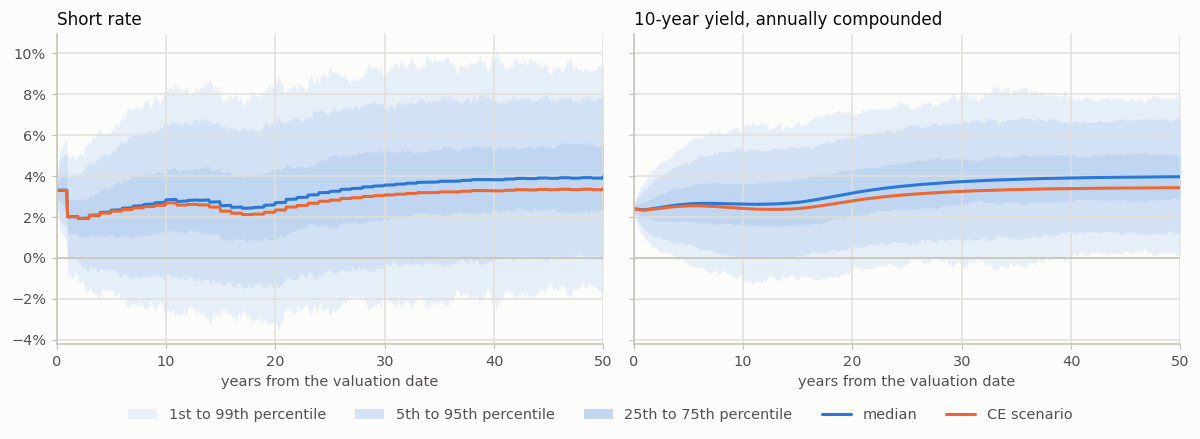
fan charts of short rates and 10-year yields,
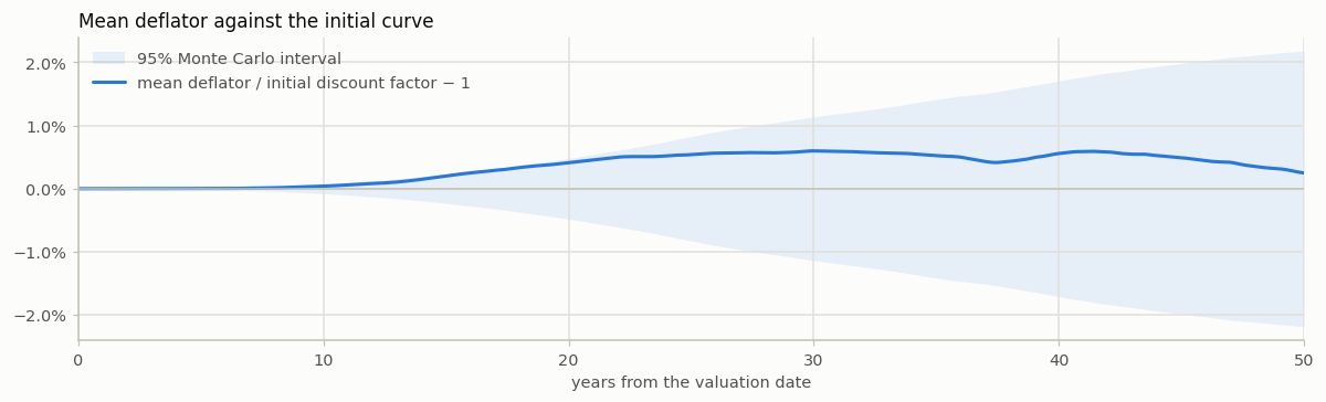
a check that the deflators reproduce the initial curve,
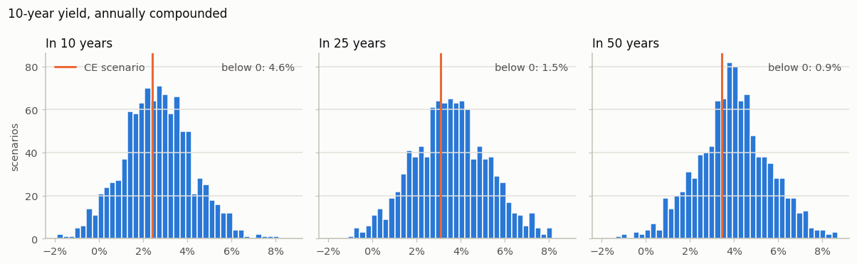
the distribution of the 10-year yield at three horizons,
the bond fund that drives the liability model,
the summary of the
Validationspace.
The model reads g2pp_input.xlsx from the library folder, which holds this notebook; edit the workbook there and run all cells again to see another input.
Click the badge below to run this notebook online on Google Colab. You need a Google account and need to be logged in to it to run this notebook on Google Colab. 
The next code cell below is relevant only when you run this notebook on Google Colab. It installs lifelib and creates a copy of the library for this notebook.
[1]:
import sys, os

if 'google.colab' in sys.modules:
    lib = 'economic'; lib_dir = '/content/'+ lib
    if not os.path.exists(lib_dir):
        !pip install lifelib
        import lifelib; lifelib.create(lib, lib_dir)

    %cd $lib_dir
[2]:
import matplotlib.pyplot as plt
import modelx as mx
import numpy as np
import pandas as pd
from matplotlib.patches import Patch
from matplotlib.lines import Line2D
from matplotlib.ticker import PercentFormatter

model = mx.read_model("BasicG2PP")
g2pp, validation = model.G2PP, model.Validation
N, n = g2pp.scen_size(), g2pp.step_size()
years = np.arange(n + 1) / 12
print(f"{N:,} stochastic scenarios plus the CE scenario, {n} months ({n / 12:g} years)")
1,000 stochastic scenarios plus the CE scenario, 600 months (50 years)
[3]:
# Chart style: light-mode tokens of the reference palette, slot 1 (blue) for the
# stochastic scenarios and slot 2 (orange) for the certainty-equivalent (CE) scenario.
SURFACE, INK, INK_2, MUTED = "#fcfcfb", "#0b0b0b", "#52514e", "#898781"
GRID, AXIS = "#e1e0d9", "#c3c2b7"
BLUE, ORANGE = "#2a78d6", "#eb6834"
plt.rcParams.update({
    "figure.facecolor": SURFACE, "axes.facecolor": SURFACE, "savefig.facecolor": SURFACE,
    "axes.edgecolor": AXIS, "axes.linewidth": 1, "axes.grid": True, "grid.color": GRID,
    "grid.linewidth": 1, "axes.spines.top": False, "axes.spines.right": False,
    "axes.labelcolor": INK_2, "axes.titlecolor": INK, "axes.titlesize": 11,
    "axes.titlelocation": "left", "xtick.color": AXIS, "ytick.color": AXIS,
    "xtick.labelcolor": INK_2, "ytick.labelcolor": INK_2, "legend.frameon": False,
    "legend.labelcolor": INK_2, "lines.linewidth": 2, "lines.solid_capstyle": "round",
    "figure.dpi": 110, "font.size": 9.5,
})

BANDS = [("1st", 1, "99th", 99), ("5th", 5, "95th", 95), ("25th", 25, "75th", 75)]
WASH = 0.10                              # nested percentile bands, each a 10% wash


def fan(ax, paths, x):
    """Percentile bands and median of the stochastic rows of paths, and the CE row."""
    stochastic = paths[1:]
    for _, lo, _, hi in BANDS:
        ax.fill_between(x, np.percentile(stochastic, lo, axis=0),
                        np.percentile(stochastic, hi, axis=0),
                        color=BLUE, alpha=WASH, linewidth=0)
    ax.plot(x, np.median(stochastic, axis=0), color=BLUE)
    ax.plot(x, paths[0], color=ORANGE)


def fan_legend(target, **kwargs):
    """Legend for fan() on an axes or a figure; nested bands show the opacity they build up to."""
    handles = [Patch(color=BLUE, alpha=1 - (1 - WASH) ** k, linewidth=0,
                     label=f"{lo} to {hi} percentile")
               for k, (lo, _, hi, _) in enumerate(BANDS, start=1)]
    handles += [Line2D([], [], color=BLUE, label="median"),
                Line2D([], [], color=ORANGE, label="CE scenario")]
    target.legend(handles=handles, **kwargs)


def percentile_table(paths, at_years, scale=100, decimals=2):
    """Table view of a fan chart: CE value and percentiles at the given years."""
    idx = [int(round(y * 12)) for y in at_years]
    stochastic = paths[1:, idx]
    table = pd.DataFrame({f"p{q}": np.percentile(stochastic, q, axis=0)
                          for q in (1, 5, 25, 50, 75, 95, 99)},
                         index=pd.Index(at_years, name="year"))
    table.insert(0, "CE", paths[0, idx])
    return (scale * table).round(decimals)
Inputs#
The run settings and G2++ parameters from the Params sheet, a few points of the selected curve, and the selected fund. The example G2++ parameters are illustrative, not calibrated.
[4]:
display(g2pp.param_table().to_frame("value"))
curve = g2pp.curve_table()[g2pp.curve_id()].dropna()
shown = [m for m in (1, 5, 10, 20, 30, 50, 100, 150) if m in curve.index]
print(f"Curve {g2pp.curve_id()}, {g2pp.compounding()} compounding, spot rates in %:")
display((100 * curve.loc[shown]).round(3).to_frame("spot rate (%)"))
print(f"Fund {g2pp.fund_id()}: {g2pp.fund_cash_share():.0%} cash, and bonds by months to maturity:")
display(g2pp.fund_bond_shares().to_frame("share"))
| value | |
|---|---|
| parameter | |
| a | 0.773 |
| b | 0.082 |
| sigma | 0.022 |
| eta | 0.0104 |
| rho | -0.7 |
| scen_size | 1000 |
| step_size | 600 |
| seed | 1234 |
| antithetic | True |
| curve_id | EUR_BASE |
| compounding | annual |
| fund_id | BOND_MIX |
Curve EUR_BASE, annual compounding, spot rates in %:
| spot rate (%) | |
|---|---|
| maturity | |
| 1.0 | 3.357 |
| 5.0 | 2.323 |
| 10.0 | 2.393 |
| 20.0 | 2.406 |
| 30.0 | 2.534 |
| 50.0 | 2.847 |
| 100.0 | 3.145 |
| 150.0 | 3.247 |
Fund BOND_MIX: 20% cash, and bonds by months to maturity:
| share | |
|---|---|
| months | |
| 60 | 0.3 |
| 120 | 0.5 |
Short rates and 10-year yields#
Each band holds the given share of the stochastic scenarios at each month. The CE scenario follows the initial forward curve. The input curve has annual maturities and flat forwards between them, so the CE short rate, and with it the median, steps at whole years. The median of the short rate sits above the forward by the convexity terms in φ(t).
[5]:
short = g2pp.short_rate_paths()
yield10 = g2pp.spot_rate_paths(120)

fig, axes = plt.subplots(1, 2, figsize=(11, 4), sharey=True)
for ax, paths, title in [(axes[0], short, "Short rate"),
                         (axes[1], yield10, "10-year yield, annually compounded")]:
    fan(ax, paths, years)
    ax.axhline(0, color=AXIS, linewidth=1)
    ax.set_title(title)
    ax.set_xlabel("years from the valuation date")
    ax.set_xlim(0, years[-1])
    ax.yaxis.set_major_formatter(PercentFormatter(1.0, decimals=0))
fan_legend(fig, loc="lower center", ncols=5, bbox_to_anchor=(0.5, 0))
fig.tight_layout(rect=(0, 0.07, 1, 1))
plt.show()
[6]:
at = [y for y in (1, 5, 10, 20, 30, 50, 100, 150) if y * 12 <= n]
print("Short rate (%): the CE value and percentiles of the stochastic scenarios")
display(percentile_table(short, at))
print("10-year yield (%)")
display(percentile_table(yield10, at))
Short rate (%): the CE value and percentiles of the stochastic scenarios
| CE | p1 | p5 | p25 | p50 | p75 | p95 | p99 | |
|---|---|---|---|---|---|---|---|---|
| year | ||||||||
| 1 | 2.01 | -0.69 | 0.06 | 1.25 | 2.01 | 2.77 | 3.96 | 4.71 |
| 5 | 2.28 | -1.51 | -0.54 | 1.17 | 2.33 | 3.49 | 5.20 | 6.17 |
| 10 | 2.69 | -2.68 | -0.89 | 1.29 | 2.84 | 4.39 | 6.56 | 8.35 |
| 20 | 2.34 | -3.17 | -1.10 | 1.06 | 2.70 | 4.34 | 6.49 | 8.56 |
| 30 | 3.08 | -2.09 | -0.16 | 1.83 | 3.56 | 5.29 | 7.27 | 9.20 |
| 50 | 3.40 | -1.54 | 0.12 | 2.38 | 3.97 | 5.56 | 7.82 | 9.48 |
10-year yield (%)
| CE | p1 | p5 | p25 | p50 | p75 | p95 | p99 | |
|---|---|---|---|---|---|---|---|---|
| year | ||||||||
| 1 | 2.33 | 1.00 | 1.38 | 1.97 | 2.35 | 2.72 | 3.32 | 3.71 |
| 5 | 2.54 | -0.30 | 0.74 | 1.80 | 2.64 | 3.49 | 4.58 | 5.67 |
| 10 | 2.42 | -0.93 | 0.02 | 1.62 | 2.63 | 3.65 | 5.30 | 6.31 |
| 20 | 2.79 | -0.62 | 0.48 | 2.00 | 3.17 | 4.35 | 5.93 | 7.11 |
| 30 | 3.25 | -0.46 | 0.95 | 2.55 | 3.73 | 4.91 | 6.58 | 8.09 |
| 50 | 3.43 | 0.15 | 1.23 | 2.95 | 3.97 | 4.99 | 6.79 | 7.93 |
The deflators reproduce the initial curve#
The mean deflator over the stochastic scenarios, divided by the initial discount factor, should be 1 at every month: E[D(t)] = P^M(0, t). The band is the 95% Monte Carlo interval, from the standard errors of antithetic pair means in Validation.martingale_test(). It widens with the horizon, because the deflators spread out as the variance V(0, t) of the integrated short rate grows.
[7]:
mart = validation.martingale_test()
ratio = mart["mc"] / mart["theory"] - 1
half_width = 1.96 * mart["se"] / mart["theory"]

fig, ax = plt.subplots(figsize=(11, 3.4))
ax.fill_between(years, -half_width, half_width, color=BLUE, alpha=WASH, linewidth=0,
                label="95% Monte Carlo interval")
ax.plot(years, ratio, color=BLUE, label="mean deflator / initial discount factor − 1")
ax.axhline(0, color=AXIS, linewidth=1)
ax.set_title("Mean deflator against the initial curve")
ax.set_xlabel("years from the valuation date")
ax.set_xlim(0, years[-1])
ax.yaxis.set_major_formatter(PercentFormatter(1.0, decimals=1))
ax.legend(loc="upper left")
fig.tight_layout()
plt.show()
print(f"largest |z| over {len(mart) - 1} months: {mart['z'].abs().max():.2f}")
largest |z| over 600 months: 1.79
Distribution of the 10-year yield#
The Gaussian model gives normally distributed yields, so a share of scenarios has negative rates; each panel prints that share.
[8]:
horizons = [y for y in (10, 25, 50) if y * 12 <= n]
values = yield10[1:, [12 * y for y in horizons]]
bins = np.linspace(np.percentile(values, 0.1), np.percentile(values, 99.9), 41)

fig, axes = plt.subplots(1, len(horizons), figsize=(11, 3.4), sharex=True, sharey=True)
for ax, horizon in zip(np.atleast_1d(axes), horizons):
    i = 12 * horizon
    ax.hist(yield10[1:, i], bins=bins, color=BLUE, edgecolor=SURFACE, linewidth=1)
    ax.axvline(yield10[0, i], color=ORANGE, label="CE scenario")
    ax.text(0.97, 0.95, f"below 0: {(yield10[1:, i] < 0).mean():.1%}",
            transform=ax.transAxes, ha="right", va="top", color=INK_2)
    ax.set_title(f"In {horizon} years")
    ax.grid(axis="x", visible=False)
    ax.xaxis.set_major_formatter(PercentFormatter(1.0, decimals=0))
first = np.atleast_1d(axes)[0]
first.set_ylabel("scenarios")
first.legend(loc="upper left")
fig.suptitle("10-year yield, annually compounded", x=0.01, ha="left", color=INK, fontsize=11)
fig.tight_layout()
plt.show()
The bond fund#
The liability model’s fund holds the shares of the Fund sheet: zero-coupon bonds by years to maturity, rebalanced monthly, plus cash. The left panel shows the growth of 1 invested at time 0. Because the fund holds only bonds and the bank account, its deflated value is a martingale; the right panel checks that its mean stays at 1.
[9]:
returns = g2pp.fund_return_paths()
growth = np.cumprod(np.hstack([np.ones((N + 1, 1)), 1 + returns]), axis=1)
fund_mart = validation.fund_martingale_test()

fig, (left, right) = plt.subplots(1, 2, figsize=(11, 4))
fan(left, growth, years)
left.set_title(f"Growth of 1 in fund {g2pp.fund_id()}")
left.set_xlabel("years from the valuation date")
left.set_xlim(0, years[-1])
fan_legend(left, loc="upper left")

half_width = 1.96 * fund_mart["se"]
right.fill_between(years, -half_width, half_width, color=BLUE, alpha=WASH, linewidth=0,
                   label="95% Monte Carlo interval")
right.plot(years, fund_mart["mc"] - 1, color=BLUE, label="mean deflated fund value − 1")
right.axhline(0, color=AXIS, linewidth=1)
right.set_title("Deflated fund value against 1")
right.set_xlabel("years from the valuation date")
right.set_xlim(0, years[-1])
right.yaxis.set_major_formatter(PercentFormatter(1.0, decimals=1))
right.legend(loc="upper left")
fig.tight_layout()
plt.show()

print(f"Growth of 1 in fund {g2pp.fund_id()}: the CE value and percentiles")
display(percentile_table(growth, at, scale=1, decimals=3))
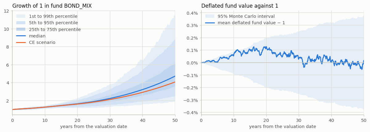
Growth of 1 in fund BOND_MIX: the CE value and percentiles
| CE | p1 | p5 | p25 | p50 | p75 | p95 | p99 | |
|---|---|---|---|---|---|---|---|---|
| year | ||||||||
| 1 | 1.034 | 0.952 | 0.974 | 1.009 | 1.033 | 1.057 | 1.096 | 1.121 |
| 5 | 1.122 | 0.974 | 1.018 | 1.075 | 1.119 | 1.165 | 1.231 | 1.285 |
| 10 | 1.267 | 1.101 | 1.144 | 1.211 | 1.266 | 1.322 | 1.400 | 1.454 |
| 20 | 1.609 | 1.179 | 1.300 | 1.490 | 1.640 | 1.803 | 2.067 | 2.278 |
| 30 | 2.119 | 1.317 | 1.528 | 1.897 | 2.239 | 2.643 | 3.279 | 3.807 |
| 50 | 4.070 | 1.949 | 2.507 | 3.597 | 4.725 | 6.196 | 8.904 | 11.479 |
Validation summary#
Each test compares Monte Carlo estimates with the values they should converge to, as z-scores. A test with m z-scores passes if its largest |z| is below the limit Φ⁻¹(1 − 0.00135/m): the same 0.27% chance of a false alarm as a single 3-sigma check, so the limit is 3 for one check and about 4.6 for 600 months. A test whose estimate is exact by construction scores 0. For a new calibration, run this with scen_size set to 10,000.
[10]:
validation.summary()
[10]:
| checks | max_abs_z | limit | ok | at | |
|---|---|---|---|---|---|
| martingale_test() | 601 | 1.790468 | 4.587190 | True | 198 |
| fund_martingale_test() | 601 | 2.043954 | 4.587190 | True | 134 |
| curve_fit_test() | 50 | 1.789351 | 4.037604 | True | 17.0 |
| moments_test() | 350 | 2.902763 | 4.472964 | True | (468, cov xy) |
| zcb_martingale_test(300, 360) | 1 | 0.941041 | 2.999977 | True | (300, 360) |
| zbp_mc(300, 360, at the money) | 1 | 0.108391 | 2.999977 | True | (300, 360, 0.8632293178757527) |
| deflator_call_test(300, 0.9) | 1 | 1.359685 | 2.999977 | True | (300, 0.9) |