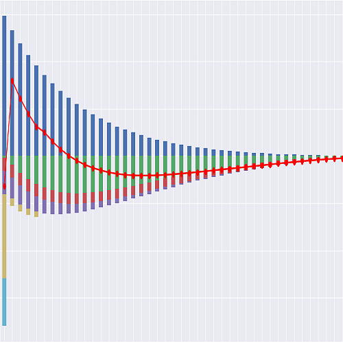
The Projection Space#
The by-policy monthly projection of the UL_US_SEC model.
The Space is parameterized by idx, the position of a model point in the table and in
every Data vector, as basiclife.BasicTerm_SC is: Projection[5]
is an ItemSpace projecting the table’s sixth row, model point 6, UL_US_S’s in-force
point restated six months on, in force 126 months at the valuation date with its loan,
and point_id() is its label:
>>> Projection[5].result_cf()          # one row per month from the valuation date
>>> Projection[5].result_av()          # the account value roll-forward behind it
>>> Projection[5].point_id()           # 6, the row's point_id
>>> Projection.idx = 1                 # or switch the default, before it computes
Compiled, no cache is ever cleared: set idx, like every Reference, on a model just
imported, before anything is computed, or project through Projection[i]. modelx
recomputes what a Reference reaches when it is set; a compiled ItemSpace takes the
References when it is made and keeps every value it has computed until it is deleted,
and the base Projection and Data keep theirs for good. And it holds each Reference
as a C variable of its shipped value’s type: a float set on an int Reference truncates
toward zero, and an int set on a float Reference reads as a float
(products/universal_life/model-sec.md, What it refuses).
Any idx makes an ItemSpace, and none is refused here. Projection[-1] reads every
vector at its last element, as numpy and a compiled memoryview both do, so it is the
table’s last point, under that point’s own point_id(); an idx past the last
row raises IndexError at its first read of a vector, which modelx reports inside its
FormulaError.
This is UL_US_S taught to run in force at a valuation date, as lifelib’s
basiclife.BasicTerm_SE extends basiclife.BasicTerm_S, and then made to compile, as
basiclife.BasicTerm_SC is made from basiclife.BasicTerm_S. A formula of
UL_US_S is rewritten where it depends on where the projection starts, where it
must answer for a month outside cover, or where it reads a table at a policy year or an
attained age; every other is UL_US_S’s own.
products/universal_life/model-sec.md lists the rewritten cells with the reason for
each. Making it compile changed how each cell reads its inputs and spells its codes, and
no number: every model point attribute a projection cell uses is read as a number from a
Data vector, every table as an array indexed by integers, every timing and kind is an
int code (Codes, below), UL_US_S’s coi_rate_scale, a Series, is a schedule
number, coi_schedule(), and UL_US_S’s claims(t, kind=None) is two
cells and their total.
Input data
Inputs are external files: plain CSVs living in the model folder’s parent
directory, products/universal_life/, read at run time rather than stored inside
the model. The model folder therefore holds nothing but formulas – no _data/, no
IOSpec, no embedded values – so a diff of the model shows logic changes only, and an
input can be edited or swapped without rewriting the model. This follows
annuallife.TradLife_A; contrast basiclife.BasicTerm_S, which keeps its inputs
inside the model through modelx’s IOSpec machinery.
The consequence worth knowing: the model is not portable on its own. Copying the
UL_US_SEC folder without its parent’s CSVs produces a model that reads and
then fails on first evaluation.
The readers live in the unparameterized Data Space, reached
here through the data Reference, so each file is read once per model rather than
once per model point. The seven assumption tables are the files UL_US_S reads,
read in place; the model point table is this model’s own:
Reference (on Data) |
Cells |
File |
|---|---|---|
model_point_file |
data.model_point_table() |
model_point_table_sec.csv |
coi_rates_file |
data.coi_rates() |
coi_rates.csv |
corridor_file |
data.corridor_factors() |
corridor_factors.csv |
mort_table_file |
data.mort_table() |
mort_table.csv |
class_factor_file |
data.class_factor_table() |
class_factor_table.csv |
lapse_table_file |
data.lapse_table() |
lapse_table.csv |
prem_persistency_file |
data.prem_persistency_table() |
prem_persistency.csv |
surr_charge_file |
data.surr_charge_table() |
surr_charge_table.csv |
Two clocks
t counts months from the valuation date, 0-based, the clock
basiclife.BasicTerm_SE runs on: t = 0 is the valuation month for every model
point, however old the policy, month t runs from the monthiversary at time t to
the next, and the frame is t = 0, 1, ..., proj_len() - 1, where proj_len()
counts the months from the valuation date to the end of the projection. Row t is the
same month for every point, so the frames of a block line up and sum row by row.
duration_mth(t) counts policy months, the months the policy has been in force at
time t: duration_mth(t) = duration_mth_init() + t, where duration_mth_init()
is read from the model point – positive for a policy in force at the valuation date, in
any month of its policy year, 0 for one issued at it, -k for one issued k months
later, at most ten years later. It is the notes’ d(t), and everything contractual
reads it: the surrender charge run-off, the COI, per-unit and premium persistency scales
by policy year, the corridor factor and the mortality rate by attained age, the first
withdrawal year, and the GPT and 7-pay limits. The policy year is the 1-based contractual
label policy_year(t) = duration(t) + 1 and the attained age (ANB) is
age(t) = age_at_entry() + duration(t), both derived and never indexed by. Point 3,
UL_US_S’s in-force cell, is in policy year 11 at attained age 45 at t = 0, and
point 9, to be issued 25 months after the valuation date, is issued at t = 25.
UL_US_S already counts its months from the start of its own projection rather than
from issue, and opens its in-force point 3 there with its account value and its loan.
What the valuation clock adds is that t = 0 is one instant for every point, that a
point may be issued after it, and that a point in force brings in what its past has left
it: the face its withdrawals have left, the year’s free allowance it has used, the
premiums it has paid and its MEC latch, four more opening values than UL_US_S reads.
The economic inputs read the valuation clock: the declared rates,
crediting_rate_ann() and comp_rate_ann(), flat as shipped, and expense
inflation, inflation_factor(t) = (1 + inflation_rate)^(t // 12), UL_US_S’s step
by year moved onto t, so that the maintenance expense is in valuation-date dollars for
every point alike. Acquisition is charged per policy issued, in the issue month, and is
not inflated, as in basiclife.BasicTerm_SE.
On a point issued at t = 0 the two clocks coincide and this model computes what
UL_US_S computes: every cell the two share agrees at every argument
UL_US_S evaluates in its sweep, but for three whose meaning changed,
pols_if_init, now the count already in force at the valuation date, model_point,
a row of another table, and result_pols, which gains the month’s new business, and
coi_rate_scale, which this model replaces with coi_schedule(). S’s claims(t,
kind) is claims_death() and claims_lapse() here, and its total,
claims(t, None), is claims(). That
is how UL_US_S’s goldens on its new-business points carry over, the worked
example among them, and tests/test_model_conventions.py asserts it cell by cell. On
point 3 the projection is UL_US_S’s, month for month, its expenses apart, which
are in valuation-date dollars.
The value state variables are closing balances at the end of month t:
av_pp(t), loan_bal_pp(t) and cum_prem_pp(t). sum_assured_at(t) is not a
closing balance: it is the face amount in force during month t, after that
month’s BOM withdrawal reduction – the face that db_pp(t), net_amt_at_risk(t)
and units(t) are measured on. wd_used_year(t) is the free allowance used in the
policy year before month t’s withdrawal, and is_mec(t) the 7-pay latch after
month t’s test. The opening values – the notes’ AV(t-1), L(t-1),
CumPrem(t-1) – are av_pp_at(t, BEF_PREM), loan_bal_pp_bom(t) and
cum_prem_pp(t - 1), and at t_entry(), the first month on the books, each chain
opens from the model point’s opening state instead, so that nothing is ever asked for a
month before the valuation date or before issue. For a point in force the opening state
is six columns of its row, per policy, as the policy stands at the start of month 0,
before any month-0 event: the account value and the loan, UL_US_S’s own columns
(av_pp_init(), loan_bal_init()); the face in force
(sum_assured_init()); the free withdrawal allowance already used in the policy year
under way (wd_used_year_init()); the premiums less withdrawals paid to date
(cum_prem_init()); and the MEC latch (is_mec_init()). UL_US_S takes the
last four as they stand at issue, the face at issue and nothing used, paid or failed, on
its in-force point too. For a point issued at or after the valuation date every one of
them is 0, and the issue values come from the formulas: sum_assured() for the face,
0 for the rest.
Every chain is one cell a month. av_pp_at(t, BEF_PREM) forms the previous month’s
close itself, from its own value at t - 1 and month t - 1’s net premium,
withdrawal, fee, deduction and interest, the same sum in the same order as
av_pp(t - 1), rather than calling for it, where UL_US_S’s account value chain ran
through five cells a month; loan_bal_pp_bom() does the same for the loan, where
UL_US_S’s ran through two, and the BEF_NB timing of pols_if_at() for the
count, one cell a month as UL_US_S’s pols_if() already was. The face, the year’s
withdrawal usage and the cumulative premium call themselves at t - 1 before anything
else, and the MEC latch does once its in-year test has run. A compiled model runs these
chains on the C stack.
Within each month the notes’ monthiversary order is followed exactly:
amortize the surrender charge (
surr_charge_rate());gross premium and its load, net premium to the account value (
premium_pp(),prem_to_av_pp());withdrawal and withdrawal fee, and under Option A the face reduction they force (
wd_pp(),wd_fee_pp(),sum_assured_at()) – after which the account value is the notes’AV'(t),av_pp_at(t, BEF_FEE);death benefit and the GPT corridor test (
db_pp());net amount at risk, the death benefit discounted one month at the guaranteed rate less the account value measured before the deduction (
net_amt_at_risk());the monthly deduction (
mth_deduction_pp());the shortfall test (
is_shortfall());end of month: one month’s interest on the post-deduction balance (
inv_income_pp()) and loan interest accrual (loan_bal_pp());end of month: decrements, death before lapse (
pols_death(),pols_lapse()).
Cash flows are undiscounted. Premiums, expenses and premium taxes fall at BOM and
are weighted by pols_if(t); death claims by pols_if(t) * mort_rate_mth(t);
surrender payments by pols_if(t) * (1 - mort_rate_mth(t)) * lapse_rate_mth(t).
Partial withdrawals also fall at BOM and are weighted by pols_if(t), but they are
withdrawals(), a cash flow line of their own rather than a kind of
claim_pp().
Counts
pols_if(t) is the count that weights row t: pols_if_at(t, BEF_DECR), the
count carried in from t - 1 (BEF_NB) plus the month’s new business,
pols_new_biz(), before the month’s decrements. A point in force at the valuation
date opens with pols_if_init(), its policy_count; one issued at or after the
valuation date opens with none, and takes its policy_count as new business in its
issue month. The recursion’s base is t_entry(), and before issue
(is_active()) every count, and so every cash flow, is zero, and so is every value
state. UL_US_S already names three timings, in a cell that returns pols_if(t) for
each and that nothing calls. BEF_DECR keeps that meaning, and so does BEF_MAT,
the count before any maturity, since nothing matures: the name keeps its S model’s
meaning, as in the family’s other models, and basiclife.BasicTerm_SE’s start-of-month
BEF_MAT is not adopted. BEF_NB is the one timing this model gives a new
meaning, basiclife.BasicTerm_SE’s, and it differs from UL_US_S’s only in the issue
month, where it counts the issued policies as new business, not yet in. Inside the month
the decrements are UL_US_S’s, death before lapse.
The end of the projection
The frame ends at omega_mth(), where the mortality table ends, and not at an event
of the contract, which never matures. With the shipped table – an annual rate of 1.0 at
ages 119 and 120 – and a class factor and an A/E of 1 or more, every life has died by
the end of the first month at attained age 119. With a preferred class, an A/E below 1,
or a table that stays below 1, lives survive the last month, and the roll-forwards read
them: check_av_roll_fwd() and av_change() read the opening account value in
force of month t + 1, which in the last month is t = proj_len(). So the two
opening values they read there, the count (the BEF_NB timing of
pols_if_at(), and through it pols_if()) and the account value
(av_pp_at(t, BEF_PREM)), are defined for 0 <= duration_mth(t) <= omega_mth():
on the books, and in the month after the frame, where they are the survivors of the last
month and the account value they carry. Both equal UL_US_S’s values there
exactly. Every other cell is zero or false there, as before issue: the account value
inside the month, the loan, every charge, premium, withdrawal, decrement rate, decrement,
claim and flow, and the expenses, whose maintenance would otherwise fall on the carried
count; only the two clocks, the inputs read on the valuation clock and the lapse shock’s
neutral 1.0 hold values there.
And nothing reads past t = proj_len(): av_change() and the two checks’ residual
cells, which read t + 1, are zero outside cover before they read it.
Naming
Cell names follow lifelib’s basiclife.BasicTerm_S and savings.CashValue_SE
wherever those models have an analogue – pols_* for policy counts, av_* for
account values, plural nouns for cash flows, *_rate for rates, *_pp for
per-policy amounts, timing and kind arguments. What running in force adds
is named as basiclife.BasicTerm_SE names it: duration_mth read from the model
point, policy_count, pols_new_biz, pols_if_at with its BEF_NB timing,
is_active and result_pols. t_entry, the first month on the books, is the SEC
models’ own, and omega_mth this model’s, named for omega_age, where the
projection ends, since the contract has no end of its own. A column of the opening state
is the cell it opens with _init added, in UL_US_S’s spelling of the stem:
av_pp_init and loan_bal_init are UL_US_S’s own, sum_assured_init,
wd_used_year_init and is_mec_init are new, and cum_prem_init is
ULSG_US_S’s name for the same column. wd_used_year already says it restarts each
policy year, so its column takes no _ytd. A table read at a policy year has one
reader keyed by the year, <cell>_py(y), and a table read at an attained age one keyed
by the age, <cell>_at(a); the monthly cell keeps UL_US_S’s name and calls it
inside cover. The surrender-charge schedule, keyed by its ID, has one reader for each of
its two columns, surr_charge_rate_max() and surr_charge_runoff_years(), and
the COI scale, keyed by sex, class and issue age, is numbered, coi_schedule(). A
check’s residual in month t is <check>_resid(t). A text column a monthly cell
branches on is read through bool decodes, one for each value it branches on, named for
the value:
is_db_option_a() and is_db_option_b(), is_gpt(), and
is_level_premium(), is_single_premium() and is_target_premium(). No
projection cell reads text: Data decodes each column into its flags, and joins the
class factor, the COI scale and the surrender-charge schedule to the points by their text
keys, so UL_US_S’s label accessors are kept for reporting alone (Reporting cells,
below). Each of UL_US_S’s claim kinds is a cell, claims_<kind>(t), and
claims() their total, as in the family’s other compiled models.
The technical notes use compact actuarial symbols instead. The mapping is:
Notes symbol |
Cells |
Meaning |
|---|---|---|
t |
(the |
Months from the valuation date |
d(t) |
duration_mth(t) |
Completed policy months at month t, the notes’ month index |
y |
policy_year(t) |
Policy year, d(t) // 12 + 1 |
(y - 1) |
duration(t) |
Completed policy years |
(none) |
point_id |
The row’s label, at idx |
x / issue_age |
age_at_entry |
Issue age (ANB) |
x + y - 1 |
age(t) |
Attained age (ANB) |
proj_len |
proj_len |
Months from the valuation date to the end of the projection |
(table’s last age) |
omega_age |
Last age of the table, 120 |
(projection end) |
omega_mth |
Policy month the projection ends at, attained age 121 |
(none) |
t_entry |
First month on the books |
(none) |
is_active(t) |
Whether month t is in cover |
sex |
sex |
Sex, M or F |
risk_class |
rate_class |
Underwriting class, one of six |
F / face_amount |
sum_assured |
Initial total face amount |
F(t) |
sum_assured_at(t) |
Total face after reductions |
(opening F) |
sum_assured_init |
Face in force entering month 0 |
U |
units(t) |
Face in $1,000 units |
db_option |
db_option |
Death benefit option, A or B |
(Option A) |
is_db_option_a |
Whether db_option is A |
(Option B) |
is_db_option_b |
Whether db_option is B |
qual_test |
qual_test |
7702 test elected; GPT only |
(GPT elected) |
is_gpt |
Whether qual_test is GPT |
premium_pattern |
premium_type |
LEVEL / SINGLE / TARGET |
(LEVEL pattern) |
is_level_premium |
Whether premium_type is LEVEL |
(SINGLE pattern) |
is_single_premium |
Whether it is SINGLE |
(TARGET pattern) |
is_target_premium |
Whether it is TARGET |
premium_mode |
(not modelled) |
Monthly premiums only [std] |
planned_premium_annual |
premium_pp_ann |
Planned annual premium |
av_initial |
av_pp_init |
Account value entering month 0 |
loan_balance_initial |
loan_bal_init |
Loan balance entering month 0 |
policy_month_offset |
duration_mth_init |
Completed policy months at the valuation date; -k if issued k months later |
(none) |
policy_count |
Policies the model point stands for |
sc_layer_table |
surr_charge_id |
Surrender charge schedule ID |
(schedule applies) |
has_surr_charge |
Whether a schedule applies |
(initial SC per $1,000) |
surr_charge_rate_max |
The schedule’s charge before any run-off |
(run-off period) |
surr_charge_runoff_years |
The schedule’s run-off, years |
guideline_single_premium |
gsp |
GSP in the GPT limit |
guideline_level_premium |
glp |
GLP in the GPT limit |
seven_pay_premium |
seven_pay_prem |
7-pay premium, an input |
GP(t) |
premium_pp(t) |
Gross premium per policy |
pp(y) |
prem_persistency(t) |
Paid/planned factor |
(pp by year) |
prem_persistency_py(y) |
The same, keyed by policy year |
pl |
load_prem_rate |
Current premium load rate |
NP(t) |
prem_to_av_pp(t) |
Net premium to account value |
W(t) |
wd_pp(t) |
Partial withdrawal |
(planned W) |
wd_pp_mth |
The wd_pp column, a month’s W |
wf |
wd_fee_pp(t) |
Withdrawal fee ($25) |
(free amount) |
wd_free_pp(t) |
Free allowance still available |
wd_used_year |
wd_used_year(t) |
Free allowance used this year |
(opening usage) |
wd_used_year_init |
The usage entering month 0 |
(face cut) |
face_reduction_pp(t) |
Option A face reduction |
AV(t) |
av_pp(t) |
Account value, end of month |
AV(t-1) |
av_pp_at(t, BEF_PREM) |
Account value, start of month |
(after premium) |
av_pp_at(t, BEF_WD) |
Before the withdrawal |
AV’(t) |
av_pp_at(t, BEF_FEE) |
After premium and withdrawal |
(AV’(t) floored at 0) |
av_pp_db_basis(t) |
The AV’ that DB and NAAR use |
AV’(t) - MD(t) |
av_pp_at(t, BEF_INV) |
After the monthly deduction |
(aggregate AV) |
av_at(t, timing) |
Account value in force |
(none) |
av_change(t) |
Change in account value |
e_pol |
expense_pol_mth |
Per-policy charge |
e_unit(y) |
expense_unit_mth_1/_2 |
Per-unit charge |
rc(t) |
rider_charge_pp(t) |
Rider charges (0) |
(e_pol + e_unit U + rc) |
maint_fee_pp(t) |
Non-COI monthly charges |
MD(t) |
mth_deduction_pp(t) |
Monthly deduction |
(the point’s scale) |
coi_schedule |
Its row of the COI table |
q_coi_guar(s) |
coi_rate_guar(t) |
Guaranteed maximum COI rate |
(q_coi_guar by year) |
coi_rate_guar_py(y) |
The same, keyed by policy year |
(last year of the scale) |
coi_rate_last_year |
The scale’s last policy year |
q_coi(s) |
coi_rate(t) |
Current COI rate |
(COI charge) |
coi_pp(t) |
Cost of insurance charge |
NAAR(t) |
net_amt_at_risk(t) |
Net amount at risk |
DB(t) |
db_pp(t) |
Death benefit after corridor |
cf(a) |
corridor_factor(t) |
GPT corridor factor |
(cf by age) |
corridor_factor_at(a) |
The same, keyed by age |
(NAAR factor) |
naar_factor |
1 + i_gm |
i_guar |
guar_rate_ann |
Guaranteed annual rate |
i_cr |
crediting_rate_ann(t) |
Current credited annual rate |
i_m |
inv_return_mth(t) |
Monthly credited rate |
i_gm |
guar_rate_mth |
Monthly guaranteed rate |
(interest credited) |
inv_income_pp(t) |
Interest credited to AV |
earned_rate(t) |
(not modelled) |
NGE revision input, no source |
L(t) |
loan_bal_pp(t) |
Loan balance, end of month |
L(t-1) |
loan_bal_pp_bom(t) |
Loan balance, start of month |
r_L |
loan_rate_ann |
Charged loan rate |
SC(t) |
surr_charge_pp(t) |
Surrender charge |
(SC per $1,000) |
surr_charge_rate(t) |
Surrender charge rate |
CSV(t) |
csv_pp(t) |
Cash surrender value |
NCSV(t) |
ncsv_pp(t) |
Net cash surrender value |
(SC retained) |
surr_charge(t) |
Surrender charge collected |
CumPrem(t) |
cum_prem_pp(t) |
Cumulative premiums |
(opening CumPrem) |
cum_prem_init |
Premiums less withdrawals before the valuation date |
(GPT limit) |
gpt_limit(t) |
max(GSP, GLP x years) |
(GPT test) |
gpt_ok(t) |
GPT compliance flag |
(7-pay limit) |
seven_pay_limit(t) |
7-pay cumulative limit |
(MEC flag) |
is_mec(t) |
7-pay failure flag, latched |
(opening MEC flag) |
is_mec_init |
The latch entering month 0 |
(grace trigger) |
is_shortfall(t) |
AV’ - L < MD |
grace_flag(t) |
(not modelled) |
In-grace state; see below |
(cure payment) |
cure_premium_pp(t) |
3 x MD plus load |
q_m(t) |
mort_rate_mth(t) |
Monthly mortality rate |
(annual q) |
mort_rate(t) |
Annual mortality rate, capped |
(base q by age) |
mort_rate_base_at(a) |
The base table’s rate |
w_base(y) |
lapse_rate_base(t) |
Base annual lapse rate |
(w_base by year) |
lapse_rate_base_py(y) |
The same, keyed by policy year |
M_sc |
lapse_rate_sc_mult(t) |
SC-expiry lapse shock |
(shock year) |
lapse_shock_year |
Policy year of the shock |
M_rate(t) |
lapse_rate_dyn_mult(t) |
Dynamic lapse multiplier |
r_comp(t) |
comp_rate_ann(t) |
Competitor new-money rate |
w_annual(y,t) |
lapse_rate(t) |
Total annual lapse rate |
w_m(t) |
lapse_rate_mth(t) |
Monthly lapse rate |
l(t) |
pols_if(t) |
In force at start of month t |
l(0) |
pols_if_init |
In force at the valuation date |
(none) |
pols_if_at(t, BEF_NB) |
Carried in from month t - 1 |
(none) |
pols_if_at(t, BEF_DECR) |
After new business: l(t) |
(none) |
pols_if_at(t, BEF_MAT) |
Before maturity: l(t) |
(none) |
pols_new_biz(t) |
Policies issued in month t |
(deaths) |
pols_death(t) |
Deaths in month t |
(lapses) |
pols_lapse(t) |
Lapses in month t |
(none) |
pols_maturity(t) |
Maturities: always zero |
(premium income) |
premiums(t) |
Premium income |
(death claims) |
claims_death(t) |
Death claims |
(surrender outgo) |
claims_lapse(t) |
Surrender payments |
(claims) |
claims(t) |
Death and surrender claims |
(withdrawal outgo) |
withdrawals(t) |
Withdrawal payments |
(maintenance) |
expenses(t) |
Maintenance expenses |
(percent of premium) |
premium_taxes(t) |
Premium tax / %-of-premium |
NetCF(t) |
net_cf(t) |
Net liability cash flow |
(none) |
check_av_roll_fwd_resid(t) |
AV roll-forward residual |
(none) |
check_margin_resid(t) |
Margin identity residual |
(none) |
result_pols() |
Counts and decrement rates |
The table covers every symbol the notes define: the Model point attributes table, the
State variables table and the notation list, in that order, followed by the cash flow
rows; the cells running in force adds sit beside the symbols they open, key or count.
Three symbols have no cells at all, and are carried in the table as (not
modelled) so that the absence is recorded rather than silent: grace_flag(t), the
one of the notes’ ten state variables with no counterpart here, because the grace
cascade is a diagnostic and no in-grace state is held (is_shortfall());
premium_mode, because every premium in this model is monthly [std]; and
earned_rate(t), the input the notes’ optional NGE revision rule would need
(crediting_rate_ann()).
Eight names needed care.
The notes’ risk_class is rate_class() here, and the model point table column
is rate_class too. The name is taken from Term_US_S/BasicTerm_S, which
this library follows ahead of the notes wherever the two collide; rate_class also
avoids reading as Python’s class. The six classes themselves are the product
spec’s, unchanged.
l(t) in the notes is the in-force probability at the start of month t, before
that month’s decrements, with l(0) = 1; pols_if(t) is the same quantity under
BasicTerm_S’s name, after the month’s new business, so pols_if(t) = l(t). On a
point issued at t = 0, pols_if(0) is the issued count, the notes’ l(0), while
pols_if_init() is 0, the count already in force at the valuation date; on a point in
force the two are one count. The notes’ recursion l(t+1) = l(t)(1 - q_m(t))(1 - w_m(t))
is the pols_if_at(t + 1, BEF_NB) step. Every BOM cash flow is weighted by
pols_if(t), which is the notes’ own l(t) weighting; take care not to read l(t)
as an end-of-month count, which would weight every flow by the survivors of the month’s
own decrements.
The notes write the monthly deduction as MD(t) and split it into a per-policy
charge, a per-unit charge, rider charges and the COI charge. CashValue_SE calls the
non-COI part of an account-value deduction maint_fee; that name is kept here for
maint_fee_pp(), and mth_deduction_pp() is the notes’ MD(t) in full.
expenses() is something different – the insurer’s own [std] maintenance
expense of $75 per policy per year, a cash flow, not a charge against the account
value. The two must not be confused: maint_fee is income, expenses is outgo.
The surrender-charge run-off SC(t) = max(0, (9.00 - (d(t) + 1)/12) x U) counts the
current month: one twelfth of a year’s amortization is already earned in the issue
month, so the charge is $8.916667 per $1,000 in the issue month, not $9.00. The month
count in surr_charge_rate() is therefore duration_mth(t) + 1, not
duration_mth(t); using the completed months alone shifts the whole run-off by a
month.
q_coi is quoted per $1,000 of net amount at risk per month and e_unit per
$1,000 of face per month, so both are divided by 1,000 – or multiplied by
units() – before they meet a currency amount. coi_rate() is therefore not
comparable with CashValue_SE.coi_rate, which is a rate per unit of account value.
surr_charge_pp(t) is the surrender charge scheduled at month t;
surr_charge(t) is the amount actually collected from lapsing policies, which is
capped by the account value because csv_pp() is floored at zero. In the first
policy years the schedule exceeds the account value and the two differ by a lot.
The notes’ cash flow table lists “Withdrawal outgo” beside “Death claims” and
“Surrender outgo”, but a partial withdrawal is a payment made on the owner’s
election, not on a contingency, so it is not a claim here: it is withdrawals(),
its own cash flow line and its own result_cf() column, and no kind of
claim_pp() is a withdrawal. The consequence to hold on to is that
claims(), the total, is the death and surrender total only, so net_cf()
subtracts withdrawals() as a separate term. The per-policy amount
stays wd_pp(), which is the notes’ W(t).
Finally, the notes write AV'(t) for one quantity and use it for two: the balance
the monthly deduction comes out of, and the balance the death benefit and the net
amount at risk are measured against. The two coincide until a policy in permanent
shortfall drives the account value negative – which this model does not prevent,
because it does not terminate such a policy (is_shortfall()).
av_pp_at(t, BEF_FEE) is the first and stays signed;
av_pp_db_basis() is the second and is floored at zero [std], so an Option B
death benefit can never fall below the face amount.
Codes
What UL_US_S spells as text, a timing or a kind, is here an int Reference named
as the text it replaces, so that every cell takes and returns C numbers. A call site
reads as it did, less the quotes: pols_if_at(t, BEF_DECR), av_pp_at(t, BEF_FEE),
claim_pp(t, DEATH).
Reference |
Value |
Meaning |
|---|---|---|
BEF_NB |
0 |
|
BEF_DECR |
1 |
|
BEF_MAT |
2 |
|
BEF_PREM |
3 |
|
BEF_WD |
4 |
|
BEF_FEE |
5 |
|
BEF_INV |
6 |
|
EOM |
7 |
|
DEATH |
0 |
|
LAPSE |
1 |
|
MATURITY |
2 |
|
The model has two families of timing, the count’s and the account value’s, passed to
different cells, and they are numbered as one: BEF_NB 0 and BEF_DECR 1, as in
every SEC model, then the count’s third, BEF_MAT, then the account value’s in the
order of their instants within the month, EOM last. So no two timings share a code,
and a code of one family passed to the other’s cell, av_pp_at(t, BEF_NB), is refused
as any timing the cell does not take is, ValueError("invalid timing"), in both
engines, rather than read as a timing of the cell’s own. Kinds are numbered in the
order the month settles them. A code a cell takes indexes that cell’s cache, a C array
of eight codes a month for each of the five cells that take one, since every 2-D cache
of the model has one width (spec_sec.py), so codes are numbered densely from 0.
They are References, not cells, so the symbol map does not list them. Every other
Reference is named in lower case, issue_age_min and omega_age among them, two of
the contract’s bounds that the compiled model’s caches are sized from (proj_len()).
Reporting cells
model_point(), the label accessors sex(), rate_class(),
db_option(), qual_test(), premium_type() and surr_charge_id(),
the reports result_cf(), result_pols() and result_av(), and the checks
check_av_roll_fwd() and check_margin() are written for a reader and for the
comparison with UL_US_S, which has every one of them: a table row, text,
DataFrames and two verdicts. No other cell calls them: each reads the number Data
decoded from the same column instead, the decodes’ flags, the schedules and the joins
the keys select. So the row, the text and the frames stay Python when the model
compiles. A label accessor returns its column as read, text or not: a blank
surr_charge_id on a point without a charge reads as NaN, and a column of numbers as
ints, and the compiled accessor returns the same. Every other cell returns a C bint,
long long or double, and so do the two checks, which may stay Python but compile
to a bint, their verdict, as their per-month residuals, *_resid, compile to a
double.
Cells Descriptions#
- model_point()[source]#
The selected model point, its row of model_point_table_sec.csv, as a Series.
Row
idxof the table, for a reader who wants every column at once: a reporting cell (the Space docstring’s Reporting cells), which no projection cell reads. Each reads its ownDatavector instead.
- point_id()[source]#
The label of the selected model point, its
point_id, fromData.point_id.Projectionis indexed by position,idx, asbasiclife.BasicTerm_SCis; the label is what a reader finds in the table, so every refusal names it.
- age_at_entry()[source]#
The issue age (ANB) of the selected model point, from
Data.age_at_entry.The age at issue, whatever the policy’s duration at the valuation date; the attained age in month t is
age().Datareads it asUL_US_Sreads it,intof the number, so a fractional age truncates toward zero.
- sex()[source]#
The sex of the selected model point, M or F.
A reporting cell (the Space docstring):
Datajoins the COI scale by it, throughcoi_schedule(), and no projection cell reads it here.
- rate_class()[source]#
The underwriting class of the selected model point (one of six).
A reporting cell (the Space docstring):
Datajoins the class factor and the COI scale by it,class_factor()andcoi_schedule(), and no projection cell reads it here.
- sum_assured()[source]#
The initial total face amount F of the selected model point, the face at issue.
The face the surrender charge is quoted on, whatever later withdrawals cut it to [S3], and the face a point not yet in force is issued with. The face in force at the valuation date is
sum_assured_init(), and the face in force in month t issum_assured_at(). FromData.sum_assured.
- db_option()[source]#
The death benefit option:
"A"(level) or"B"(face plus account value).Option C (return of premium) is out of scope in the product spec. A reporting cell (the Space docstring):
Datadecodes the column intois_db_option_a()andis_db_option_b(), and no projection cell reads it here.
- is_db_option_a()[source]#
Whether the death benefit is Option A, the level face, from
Data.is_db_option_a.Datadecodes thedb_optioncolumn, 1 where it is"A", so that no monthly cell branches on text;db_pp()andface_reduction_pp()read this instead.
- is_db_option_b()[source]#
Whether the death benefit is Option B, the face plus the account value.
From
Data.is_db_option_b, 1 wheredb_optionis"B", read bydb_pp(), which raises on a point that is neither A nor B, asUL_US_S’s does.
- qual_test()[source]#
The IRC 7702 qualification test elected at issue; only
"GPT"is modeled.CVAT is out of scope in the product spec, so
corridor_factor()raises on anything else rather than silently applying GPT corridor factors. A reporting cell (the Space docstring):Datadecodes the column intois_gpt(), and no projection cell reads it here.
- is_gpt()[source]#
Whether the point elected the Guideline Premium Test, from
Data.is_gpt.1 where
qual_testis"GPT", read bycorridor_factor(), which raises on any other test, asUL_US_S’s does: CVAT is out of scope in the product spec.
The premium pattern:
"LEVEL","SINGLE"or"TARGET"[std].A reporting cell (the Space docstring):
Datadecodes the column intois_level_premium(),is_single_premium()andis_target_premium(), and no projection cell reads it here.
Whether the premium pattern is LEVEL, from
Data.is_level_premium.One of the three decodes of the
premium_typecolumn thatpremium_pp()branches on, so that no monthly cell compares text;premium_pp()raises on a point that is none of the three, asUL_US_S’s does.
Whether the premium pattern is SINGLE, from
Data.is_single_premium.A decode of the
premium_typecolumn, read bypremium_pp().
Whether the premium pattern is TARGET, from
Data.is_target_premium.A decode of the
premium_typecolumn, read bypremium_pp().
The planned annual premium per policy; a billing target only [S3].
From
Data.premium_pp_ann.
- wd_pp_mth()[source]#
The planned partial withdrawal per policy, in each month withdrawals are allowed.
The model point’s
wd_ppcolumn,Data.wd_pp, a monthly amount, 0 in every shipped model point: the notes give no withdrawal utilization pattern, so the behaviour is left to the data [std]. Read once a point here, so thatwd_pp(), a monthly cell on the account value’s chain, reads no table in its own formula.
- load_prem_rate()[source]#
The current premium load rate, 6% [std] (guaranteed maximum 9%) [S1].
The load is itself a non-guaranteed element in the source design, which is why it sits in the model point table rather than in a Reference. From
Data.load_prem_rate, which refuses a load outside 0 to 1.
- av_pp_init()[source]#
AV entering month 0: the account value per policy at the valuation date.
The
av_pp_initcolumn,UL_US_S’s own and the notes’av_initial: the balance at the close of policy monthduration_mth_init() - 1, before any month-0 event, which is whatUL_US_Scarries into the month asav_pp_at(d, BEF_PREM)atd = duration_mth_init(). It is the opening balance of the account value chain att_entry(),av_pp_at(0, BEF_PREM). Zero for a point not yet in force, which is issued with no account value.Datarefuses a negative one: an account value below zero is an artifact of the grace cascade the model does not implement, which no policy in force can hold. FromData.av_pp_init.
- loan_bal_init()[source]#
L entering month 0: the policy loan balance per policy at the valuation date.
The
loan_bal_initcolumn,UL_US_S’s own and the notes’loan_balance_initial: the debt outstanding at the close of policy monthduration_mth_init() - 1, interest accrued to then included, before any month-0 event. It is the opening balance ofloan_bal_pp_bom()att_entry(), the loaned portion that month 0’s interest credit, shortfall test and death claim read. Zero for a point not yet in force. FromData.loan_bal_init.
- sum_assured_init()[source]#
F entering month 0: the total face amount in force at the valuation date.
The
sum_assured_initcolumn: the face in force at the close of policy monthduration_mth_init() - 1, after every Option A withdrawal cut to date, which is the faceUL_US_Scarries into the month assum_assured_at(d - 1). It is the base ofsum_assured_at()att_entry(), so month 0’s own withdrawal cut, death benefit, net amount at risk and per-unit charge are measured from it. The face at issue,sum_assured(), stays the surrender-charge base, andDatarefuses a value above it, since face increases are not modelled. Zero for a point not yet in force, which is issued atsum_assured().UL_US_Sopens its in-force point at the face at issue. FromData.sum_assured_init.
- wd_used_year_init()[source]#
The free withdrawal allowance already used in the policy year under way, per policy.
The
wd_used_year_initcolumn: the free part of every withdrawal taken since the anniversary on or before the valuation date, through policy monthduration_mth_init() - 1, which is whatUL_US_Scarries into the month aswd_used_year(d).wd_used_year()opens from it att_entry(), so month 0’s free amount is what is left of the year’s 10%. The cell’s name already says it restarts each policy year, so the column takes no_ytd: on a point valued on an anniversary the year has just begun, the usage is 0, andDatarefuses any other value there. Zero for a point not yet in force.UL_US_Sopens its in-force point with the year’s allowance unused. FromData.wd_used_year_init.
- cum_prem_init()[source]#
CumPrem entering month 0: premiums less withdrawals per policy before the valuation.
The
cum_prem_initcolumn: every gross premiumpremium_pp()collected from issue through policy monthduration_mth_init() - 1, less every withdrawalwd_pp()paid, which is whatUL_US_Scarries into the month ascum_prem_pp(d - 1).cum_prem_pp()opens from it att_entry(), so the GPT test, the 7-pay test and the TARGET premium cap of month 0 all count the premiums paid before the valuation date.ULSG_US_Sgives the same column this name. FromData.cum_prem_init.It may be negative. The notes’ “less a portion of withdrawals” is taken as the whole withdrawal [std], so this is a tax measure, not a balance, and withdrawals can exceed the premiums paid;
Dataholds the account value, the loan, the face and the usage to zero or more, and this to a number. Zero for a point not yet in force.UL_US_Sopens its in-force point with none paid.
- is_mec_init()[source]#
The MEC latch entering month 0: whether the 7-pay test failed before it.
The
is_mec_initcolumn, an int code: 1 for a policy that failed the 7-pay test in some month before the valuation date, and so is a modified endowment contract for good, 0 otherwise. It is whatUL_US_Scarries into the month asis_mec(d - 1).is_mec()latches on it att_entry(), so a policy that failed in its first seven years stays a MEC after them, where the in-year test no longer applies.Datarefuses a 0 wherecum_prem_initalready exceeds the 7-pay limit of the month before the valuation date, inside the first seven policy years. FromData.is_mec_init, an int64 vector, so 1.0 reads as 1, and True. Zero for a point not yet in force.UL_US_Sopens its in-force point with the latch off.
- policy_count()[source]#
The number of policies the model point stands for, its
policy_countcolumn.A point in force at the valuation date counts the policies in force then, before any month-0 event; any other point counts the policies it issues. Either way the count enters the projection once: as
pols_if_init()for the first, aspols_new_biz()in the issue month for the second. Every per-policy value – the account value, the loan, the face, the opening state – is the same whatever the count, and every cash flow is a per-policy amount weighted by it. FromData.policy_count.
- pols_if_init()[source]#
Policies in force at the valuation date, before any month-0 event.
policy_count()for a point already in force att = 0(duration_mth_init() > 0), and 0 for one issued at or after it, whose policies enter throughpols_new_biz()in the issue month instead, as inbasiclife.BasicTerm_SE. So on a point issued att = 0this is 0, andpols_if(0)is the issued count.UL_US_S’s cells of the name is the notes’l(0), the count at the start of its frame, which on new business is the issued count.
- duration_mth_init()[source]#
Completed policy months at the valuation date, the
duration_mthcolumn.The policy’s age in months at
t = 0: 120 for point 3,UL_US_S’s in-force cell, 126 for point 6, the same policy six months on, 0 for a policy issued at the valuation date, and -25 for point 9, to be issued 25 months after it, whichDataadmits up tofuture_horizon_mthmonths ahead. This is the notes’policy_month_offset, an elapsed count, already 0-based, andUL_US_S’s cells and column of the same name, which count from the first projected month; here that month is the valuation date for every point, and the count may be negative. It is the one fact the policy clock takes from the model point, fromData.duration_mth.
- has_surr_charge()[source]#
Whether a surrender charge schedule applies to this model point.
From
Data.has_surr_charge, 1 where the column reads True.
- surr_charge_id()[source]#
The surrender charge schedule ID, a row label of surr_charge_table.csv.
A reporting cell (the Space docstring):
Datajoins the schedule by it, intosurr_charge_rate_max()andsurr_charge_runoff_years(), and no projection cell reads it here. A point without a charge is never refused for it, so it may be blank, read as NaN, or a number, as the column reads, and is returned as read.
- surr_charge_rate_max()[source]#
The schedule’s charge per $1,000 of initial face, before any of it runs off.
The
sc_per_1000_initcolumn of this point’s row of surr_charge_table.csv, $9.00 on the shippedUL9schedule;surr_charge_rate()amortizes it linearly from here.Data.surr_charge_rate_maxjoins it to the points bysurr_charge_id, once the table and the join are checked, so that no projection cell reads the table.surr_charge_rate()reads it only wherehas_surr_charge()is true, but a point without a charge reads its schedule too, as at stageE, where the table holds its id; where it does not,Data.has_surr_charge_scheduleis 0, and this raisesKeyError, naming the point, where stageE’s.locraised it.
- surr_charge_runoff_years()[source]#
The number of policy years over which the schedule’s charge runs off.
The
runoff_yearscolumn of this point’s row of surr_charge_table.csv, 9 on the shippedUL9schedule, read as a float:surr_charge_rate()amortizessurr_charge_rate_max()over it, andlapse_shock_year()is the year after it. Joined byData.surr_charge_runoff_yearsassurr_charge_rate_max()is, which refuses on a point with a charge a run-off of 0, whichsurr_charge_ratewould divide by, or one of2**53years or more in size, the bound every number read as an int is held to: the compiledint()inlapse_shock_year()converts it through a Python int to a Clong long, exact below2**63and raisingOverflowErrorpast it. Read by those two only wherehas_surr_charge()is true; on a point without a charge it reads the schedule where the table holds its id, as at stageE, and raisesKeyError, naming the point, where it does not, assurr_charge_rate_max()does.
- seven_pay_prem()[source]#
The 7-pay premium (IRC 7702A compliance input) [S3], from
Data.seven_pay_prem.
- duration_mth(t)[source]#
d(t): completed policy months at the beginning of month t, the policy clock.
duration_mth_init() + t:tcounts months from the valuation date andduration_mth(t)months from issue, and the two move together. A closed form, wherebasiclife.BasicTerm_SEadds one a month by recursion: the same numbers, without a call chain as long as the frame. It is 0 in the issue month,t = 0for a point issued at the valuation date, and negative before issue. This is the elapsed count in lifelib’s sense (CashValue_SE.duration_mth) and the notes’ month index; the surrender charge run-off counts the current month as well,duration_mth(t) + 1– seesurr_charge_rate().
- duration(t)[source]#
Completed policy years at the beginning of month t,
duration_mth(t) // 12.0 throughout the first policy year, and negative before issue.
- policy_year(t)[source]#
y: the policy year containing month t, the 1-based contractual label.
duration(t) + 1: derived fromt, and the key every policy-year table (coi_rates.csv, lapse_table.csv, prem_persistency.csv) is read with. It is 0 or less before issue, where no table is read by it: each reader is called inside cover only (is_active()).
- age(t)[source]#
The attained age (ANB) in month t:
age_at_entry() + duration(t).This is the notes’
x + y - 1. Age changes on the policy anniversary, not on the birthday, which is the ANB convention the whole model is built on [std]. Before issue it is below the issue age, where no table is read at it.
- omega_mth()[source]#
The policy month at which the projection ends, the first at attained age 121.
12 * (omega_age - age_at_entry() + 1): 1,032 at issue age 35. The mortality table ends atomega_age(120), where the annual rate is 1.0, so the last projected month,omega_mth() - 1, is the last at attained age 120. It isUL_US_S’s frame length, counted from issue on the policy clock;proj_len()counts from the valuation date instead. The contract has no maturity date [S2][S3], so the cell is named foromega_age, the end of the table, and not for an event of the policy: where lives survive the last month, the count and the account value they carry into this month are kept (seepols_if_at()).
- proj_len()[source]#
The number of months from the valuation date to the end of the projection.
omega_mth() - duration_mth_init(): 1,032 for a policy issued at age 35 at the valuation date, 912 for point 3, in force 120 months, and 1,057 for point 9, issued 25 months after the valuation date. The frame ist = 0, 1, ..., proj_len() - 1;proj_len()is its exclusive end, the row count ofresult_cf(), andproj_len() - 1is the last projected month, the last at attained age 120. The contract has no maturity date [S2][S3]; the projection is truncated by mortality, not by the policy.Three kinds of point have no frame the contract issues, and each raises here, naming the point, rather than projecting what the contract does not hold, in this order:
one issued above
omega_age, 120, which would never be in cover:UL_US_Sprojects it as months in which nothing happens. Checked first, so that a point to be issued there is refused whenever it is to be issued;one at or past the end of the projection at the valuation date, which an in-force extract should not carry;
one issued below
issue_age_min, 18, the youngest issue ageproduct-spec.mdadmits.UL_US_Sprojects any age its tables serve, but the compiled model’s caches are sized from the contract (spec_sec.py), so a younger point, whose frame and policy years run longer, would read past them. A fractional issue age is read asUL_US_Sreads it, truncated, so 17.5 is 17 and refused.
- t_entry()[source]#
The first month the policy is on the books:
max(0, -duration_mth_init()).0 for a point in force at the valuation date or issued at it,
kfor one issuedkmonths later. It is the base of every recursion: the count, the account value, the loan, the face, the year’s withdrawal usage, the cumulative premium and the MEC latch all open there, from the model point’s opening state on a point in force and from the issue values on any other. No cell in cover reads a month before it.
- is_active(t)[source]#
Whether month t is inside cover: issued, and inside the projection.
0 <= duration_mth(t) < omega_mth(), false before issue and fromt = proj_len()on. Outside cover every count, charge, premium, withdrawal, decrement rate, decrement, claim and flow is zero and every flag false, no table is read at a policy year or an attained age the policy does not have, and nothing reads a month pastproj_len(); the clocks and the inputs read on the valuation clock keep their values, and the lapse shock’s multiplier its neutral 1.0. The two exceptions are the opening values of the month after the frame, the count and the account value carried intot = proj_len(), which the roll-forwards read (seepols_if_at()andav_pp_at()).
- crediting_rate_ann(t)[source]#
i_cr: the current declared annual effective credited rate, 4.00% [std].
A non-guaranteed element under ASOP 2 [R8]. The base deterministic run holds the snapshot scale level, as the notes prescribe. The notes’ optional revision rule
i_cr(t) = max(i_guar, earned_rate(t) - spread)needs an earned-rate input the notes do not supply and is not implemented.An economic input, so it is read on the valuation clock:
tcounts months from the valuation date, and a declared-rate scenario would be indexed by it, one path for every point of a block, however old the policy. The shipped rate is flat, so the clock shows in no number.
- inv_return_mth(t)[source]#
i_m: the monthly credited rate,
(1 + i_cr)^(1/12) - 1.0.0032737 at the [std] 4.00% current rate. The contract credits daily on a 365-day year [S3]; monthly compounding is the model’s discretization [std] – do not also compound daily.
- naar_factor()[source]#
The specimen’s NAAR factor,
1 + i_gm= 1.0016516 [std] at 2% [S3].The death benefit is discounted one month at the guaranteed rate, never the credited rate; the specimen prints 1.0024663 = 1.03^(1/12) at its own 3% guarantee [S3].
- loan_rate_mth()[source]#
The monthly charged loan rate,
(1 + r_L)^(1/12) - 1at r_L = 2.75%.The contract accrues daily and capitalizes annually [S3]; monthly compounding is the model’s discretization [std].
- prem_persistency(t)[source]#
pp(y): the fraction of the planned premium actually paid in policy year y [std].
100% in year 1, declining 2 percentage points a year to a 70% floor from year 16, read from prem_persistency.csv at the policy year of month t by
prem_persistency_py(). The shape is informed qualitatively by the SOA/LIMRA UL study [R7]; the levels are a standardization. Zero outside cover, before the table is read: before issue the valuation clock reaches policy years 0 and below.
- prem_persistency_py(y)[source]#
pp(y) in policy year y, from prem_persistency.csv: the table’s one reader.
Data.prem_persistency_array()at the year, the table padded from year 0, so that the year is the index. Policy years beyond the table take its last row, the last yeardata.prem_persistency_last_year()gives, which it reads from the table’s key column once it has checked the keys and the factors, before any factor is read. A year below 1, before the table’s first row, whereUL_US_S’s.locraisedKeyError, is refused, naming the point and the year, so that the padding is never read. Keyed by the contractual policy year, so the table is read once a policy year rather than once a month;prem_persistency()calls it inside cover only.
GP(t): the gross premium per policy received at BOM of month t.
LEVELPlanned annual premium / 12, times
prem_persistency().SINGLEOne premium in the issue month, capped at the guideline single premium.
TARGETAs
LEVELbut capped so cumulative premium stays inside the GPT limit [std]; the cap looks at the cumulative premium before this month’s,cum_prem_pp(t - 1), so there is no circularity. In the first month on the books,t_entry(), that iscum_prem_init(), the premiums paid before the valuation date, 0 at issue: a TARGET point in force near its limit collects only what the limit still has room for.
Zero from attained age 121, when premiums are no longer accepted [S2][S3], and zero outside cover. The pattern is read through its decodes,
is_single_premium(),is_level_premium()andis_target_premium(), not as text.
Premium income at BOM of month t, weighted by the in force at BOM.
- wd_pp(t)[source]#
W(t): the partial withdrawal per policy at BOM of month t.
Withdrawals are allowed from the first policy anniversary and stop at attained age 121 [S3]. The amount is the constant monthly figure
wd_pp_mth(), the model point’swd_ppcolumn, from the valuation date on, 0 in every shipped model point: the notes give no withdrawal utilization pattern, so the mechanics are implemented and the behaviour is left to the data [std]. Zero outside cover, before either contractual test, so that nothing is withdrawn att = proj_len()whateveromega_ageandcharges_cease_ageare set to.
- wd_used_year(t)[source]#
The free-withdrawal allowance already consumed in the current policy year.
The notes’
wd_used_yearstate variable, “free-withdrawal usage in current policy year, updated on withdrawal”: reset to zero on each policy anniversary and increased month by month by the free part of each withdrawal taken since,min(W(t-1), wd_free_pp(t-1)). It is a value entering month t, before month t’s own withdrawal.This is what makes the notes’ allowance an annual one. Without it the 10% is granted afresh every month, and a policyholder withdrawing 10% of the account value every month takes twelve full annual allowances in a policy year and never triggers the Option A face reduction of
face_reduction_pp().In the first month on the books,
t_entry(), it iswd_used_year_init(), the usage of the policy year under way at the valuation date. The anniversary reset comes first, so in an anniversary month, the issue month included, it is 0 whatever the model point says, andDatarefuses a non-zero usage on a point valued on an anniversary. Zero outside cover.
- wd_free_pp(t)[source]#
The free partial withdrawal allowance still available in month t [std].
max(0, 10% of AV - wd_used_year(t)): the allowance is 10% of the account value measured after the premium and before the withdrawal, less the part of it already taken earlier in the same policy year, and it resets on each policy anniversary – the notes’ “free-amount rule (10% of AV per policy year)” with itswd_used_yearstate (wd_used_year()). In the first withdrawal month of a policy year nothing is used yet and this is the full 10%.The specimen’s carve-out is the lesser of $10,000 and 10% of net cash surrender value, on the first withdrawal of each of the first 15 policy years [S3]; the composite simplifies to 10% of the account value, with no dollar cap and no 15-year limit [std].
- wd_fee_pp(t)[source]#
wf: the $25 withdrawal fee, charged only in a month with a withdrawal [S2][S3].
The fee is retained by the insurer, so it is account-value outgo but not a liability cash flow; it appears in
margin_expense(), not inclaims().
- face_reduction_pp(t)[source]#
The total face reduction forced by a withdrawal under Option A [S3].
Under Option A a withdrawal beyond the free amount would otherwise increase the net amount at risk, so the face is cut by the excess. The free amount is whatever is left of the policy year’s allowance (
wd_free_pp()), not a fresh 10% each month. Under Option B the withdrawal reduces the account value only, and this is zero. The option is read through its decode,is_db_option_a().
- sum_assured_at(t)[source]#
F(t): the total face amount in force in month t, after any reductions.
The face entering the first month on the books,
t_entry(), is the face in force at the valuation date,sum_assured_init(), on a point in force, and the face at issue,sum_assured(), on any other; the face in monthtis the previous month’s less the reduction forced by this month’s withdrawal, soF(t)already reflects a reduction taken at BOM of montht, the first month’s included. Face increases, elective decreases and option changes are not modeled, so the only movement is the Option A withdrawal reduction. Zero outside cover.
- units(t)[source]#
U: the total face amount in $1,000 units,
sum_assured_at(t) / 1000.The per-unit charge is quoted per $1,000 of face per month, so it is multiplied by this. The surrender charge is quoted per $1,000 of initial face, because face decreases do not reduce it [S3]; see
surr_charge_pp().
- corridor_factor(t)[source]#
cf(a): the GPT corridor factor at the attained age of month t [S3][R2].
250% to age 40, grading to 101% above age 93, read by
corridor_factor_at(). Only the Guideline Premium Test is modeled; CVAT is out of scope in the product spec, so any otherqual_testraises rather than being treated as GPT, in whatever month, since it is a fault of the point; the test is read through its decode,is_gpt(). Zero outside cover, before the table is read.
- corridor_factor_at(a)[source]#
cf at attained age a, from corridor_factors.csv: the table’s one reader.
Data.corridor_factor_array()at the age, the table padded from age 0, so that the age is the index. Ages outside the table take its nearest row, which above it is 101%: the first and last agesdata.corridor_age_first()anddata.corridor_age_last()give, which they read from the table’s key column once the keys and the factors are checked, before any factor is read. So the padding is never read, and no age below 0 is either:Datarefuses a table whose first age is negative. The last is asked for first, since it runs the checks and the first is counted back from it, which keeps the call one level shallower. Keyed by the attained age, so the table is read once an age rather than once a month;corridor_factor()calls it inside cover only.
- av_pp_db_basis(t)[source]#
AV’(t) floored at zero: the balance the death benefit is measured against.
The notes’ step 4 sets the Option B death benefit to
F + AV'(t)and step 5 measures the net amount at risk against the sameAV'(t), both on the premise thatAV'is a real account balance. It stops being one as soon as a policy in permanent shortfall keeps being projected: the grace and lapse-for-insufficiency cascade is not implemented (seeis_shortfall()), so nothing terminates such a policy and its account value runs deeply negative. Fed toF + AV'unfloored that gives an Option B death benefit below the face amount, and in the end a negative one – a death claim paid by the beneficiary, which no universal life contract can produce.Flooring the balance at zero here is [std], and is the same floor
csv_pp()already carries for the same reason: a negative account balance is an artifact of the missing termination, not a contract state. It holds the Option B death benefit at or above the face amount, and it stops the net amount at risk from growing with the shortfall and charging COI on a fund that is not there.Wherever
AV'(t) >= 0– every month of model points 1 and 3, and the first 677 of point 2’s 1,032 months – this is exactlyav_pp_at(t, BEF_FEE)and changes nothing, so the worked example is untouched.
- db_pp(t)[source]#
DB(t): the death benefit per policy after the corridor test [S1][S3].
max(option_db, cf(a) x AV'(t))whereoption_dbis the face amount under Option A and face plus account value under Option B, andAV'(t)is the account value after premium and withdrawal and before the monthly deduction. Taking the account value at that point is what removes the circularity the notes warn about: under Option B the death benefit depends on the account value and the net amount at risk depends on the death benefit, but with this BOM ordering neither depends on the deduction.The
AV'(t)used here isav_pp_db_basis(), floored at zero [std], so the death benefit is never less than the face amount; see that cells for why the floor is needed at all. The option is read through its decodes,is_db_option_a()andis_db_option_b(), not as text. Zero outside cover, before the corridor table is read.
- net_amt_at_risk(t)[source]#
NAAR(t):
DB(t) / (1 + i_gm) - AV'(t), floored at zero [S3].Two conventions here are the specimen’s, not conveniences: the death benefit is discounted one month at the guaranteed rate (
naar_factor()), and the account value is measured before the monthly deduction. Using the credited rate in the discount, or the post-deduction account value, makes the COI charge implicit and requires iteration, and produces small systematic COI errors.The
AV'(t)subtracted isav_pp_db_basis(), the same floored balance the death benefit is measured on, so the two sides of the subtraction stay consistent.
- coi_schedule()[source]#
The number of this point’s guaranteed COI scale, its row of
Data.coi_rate_array.Data.coi_scheduleat this point:Datanumbers each issue-age cell of coi_rates.csv, itssex,rate_classandage_at_entry, from 1 in the order of those keys, and gives each point the number of its own, or 0 where the table has no scale for it.UL_US_Sslices the scale, a Series, by the same three keys incoi_rate_scale, which this replaces, since no compiled cell returns a Series. A point without a scale is projected asUL_US_Sprojects it while no COI rate is read, and refused bycoi_rate_last_year()once one is.
- coi_rate_guar(t)[source]#
q_coi_guar(s): the guaranteed maximum monthly COI rate per $1,000 NAAR [S3].
A 2001 CSO-era specimen table, log-linearly interpolated between the printed anchor years [std]; it grades to 1000/12 at attained ages 112-120 and to zero from attained age 121. Read at the policy year of month t by
coi_rate_guar_py(); zero outside cover, before the scale is read.
- coi_rate_guar_py(y)[source]#
q_coi_guar in policy year y, from this point’s scale: the scale’s one reader.
Data.coi_rate_array()at the point’scoi_schedule()and the year, each schedule padded from year 0, so that the year is the column. Policy years beyond the scale take its last row,coi_rate_last_year(), which is asked for first, so that a projection meets the check of the table’s keys, and the refusal of a point without a scale, before any rate is read. A year below 1, whereUL_US_S’s slice raisedKeyError, is refused, naming the point and the year, so that the padding is never read. Keyed by the contractual policy year;coi_rate_guar()calls it inside cover only.
- coi_rate_last_year()[source]#
The last policy year of this point’s guaranteed COI scale: its extent.
Data.coi_rate_last_yearsat this point, the last year of its scale, whichDatareads from the table’s key columns once it has checked the keys and the rates. 87 on the shipped anchor cell, whose scale runs to attained age 121. A point the table has no scale for, schedule 0, has a last year of 0, and is refused here, naming it, whereUL_US_S’s slice raisedKeyError: when its first COI rate is read, and not before, since a point valued, or issued, at or pastcharges_cease_agenever reads one, andUL_US_Sprojects it. The element is compared, andintof it returned, rather than held in a local first, which a formula that also builds a message would keep a Python object compiled.
- coi_rate(t)[source]#
q_coi(s): the current monthly COI rate,
coi_curr_factorx guaranteed [std].60% of the guaranteed maximum at every duration. Current COI scales are not published – only guaranteed maxima appear in the specimen [S3] – so this factor is a pure modeling assumption and one of the two assumptions to sensitivity-test first.
Note the units: this is per $1,000 of net amount at risk per month, so it is divided by 1,000 in
coi_pp(). It is not comparable withCashValue_SE.coi_rate, which is a rate per unit of account value.
- coi_pp(t)[source]#
The cost of insurance charge per policy,
q_coi(y) / 1000 x NAAR(t)[S3].Zero from attained age 121, when monthly deductions cease [S2][S3], and zero outside cover.
- rider_charge_pp(t)[source]#
rc(t): rider charges, 0 in the base model [std].
The notes carry this term in the monthly deduction so that rider modules can be added without changing the recursion [S3].
- maint_fee_pp(t)[source]#
The non-COI part of the monthly deduction per policy [S3].
e_pol + e_unit(y) x U + rc(t): the $7.50 per-policy administrative charge, the per-unit coverage charge of $0.26 per $1,000 of face per month in policy years 1-10 and $0.156 thereafter, and rider charges. Zero from attained age 121, when charges cease [S2][S3], and zero outside cover.The name follows
CashValue_SE.maint_fee: this is a charge against the account value and therefore insurer income. It is notexpenses(), which is the insurer’s own outgo.
- maint_fee(t)[source]#
Non-COI monthly charges deducted from account values, for the policies in force.
- mth_deduction_pp(t)[source]#
MD(t): the monthly deduction per policy, taken at BOM [S3].
e_pol + e_unit(y) x U + rc(t) + q_coi(y) / 1000 x NAAR(t), i.e.maint_fee_pp()pluscoi_pp(). The deduction at the start of month t pays for month t’s coverage: the specimen says the deduction provides coverage for the following policy month, which with BOM indexing is the month it is taken in.
- av_pp_at(t, timing)[source]#
Account value per policy at an intra-month point of month t.
The BOM events change the balance in this order, and
timingnames the point just before each of them:BEF_PREMBefore the premium: the closing balance of the previous month,
AV(t-1), or the model point’s opening balanceav_pp_init()in the first month on the books,t_entry()– the account value at the valuation date on a point in force, 0 at issue. This is where the opening state enters the recursion, as inCashValue_SE;av_pp()itself has no base case. The previous month’s close is formed here, from this timing’s own value att - 1and montht - 1’s net premium, withdrawal, fee, deduction and interest, the same sum in the same order asav_pp(t - 1), rather than called for, so the chain of calls back tot_entry()is one cell a month, whereUL_US_S’s ran through five. It is also defined in the month after the frame,t = proj_len(), where it is the account value the survivors of the last month carry, which the roll-forward reads; zero before issue.BEF_WDAfter the net premium, before the withdrawal.
BEF_FEEAfter the withdrawal and its fee, before the monthly deduction. This is the notes’
AV'(t), and the balance the death benefit, corridor test and net amount at risk are all measured against.BEF_INVAfter the monthly deduction, before interest. Interest is credited on this post-deduction balance; reversing the two overstates the account value by about one month’s interest on the deduction every month.
The end-of-month balance
AV(t)isav_pp(). The three timings afterBEF_PREMare zero outside cover,t = proj_len()included.
- inv_income_pp(t)[source]#
Interest credited to the account value per policy at EOM of month t.
The unloaned part of the post-deduction balance earns the current monthly rate and the loaned part earns the guaranteed monthly rate [S2][S3]:
(AV'(t) - MD(t) - L(t-1)) x i_m + L(t-1) x i_gm
which is the notes’ step 8 rearranged. The loaned portion is taken as the opening loan balance
loan_bal_pp_bom()exactly, as the notes write it, without capping it at the account value.
- av_pp(t)[source]#
AV(t): the account value per policy at the end of month t.
The post-deduction balance plus one month’s interest, for every month of the frame including the first on the books: the opening balance
av_pp_init()enters throughav_pp_at(t, BEF_PREM), not through a base case here. With no loans and no withdrawals this collapses to the notes’ core recursionAV(t) = [AV(t-1) + NP(t) - MD(t)] x (1 + i_m), which in the issue month of a point projected from issue reproduces the contractual policy-date rule that the account value equals the net premium less the first monthly deduction [S3]. Zero outside cover, through its timings.
- loan_bal_pp_bom(t)[source]#
L(t-1): the policy loan balance per policy at the beginning of month t.
The previous month’s closing balance, or the model point’s opening balance
loan_bal_init()in the first month on the books,t_entry()– the debt at the valuation date on a point in force, 0 at issue. This is the loaned portion the interest credit, the shortfall test and the death claim all read; it plays for the loan the partav_pp_at(t, BEF_PREM)plays for the account value, and like it forms the previous month’s close itself, its own value att - 1times(1 + r_L)^(1/12), the productloan_bal_pp()takes, rather than calling for it. So the chain back tot_entry()is one cell a month, whereUL_US_S’s ran through two. Zero outside cover: nothing reads the loan att = proj_len(), where it would turn the death claim on a death benefit of 0 negative.
- loan_bal_pp(t)[source]#
L(t): the policy loan balance per policy at the end of month t.
L(t-1) x (1 + r_L)^(1/12)on the opening balanceloan_bal_pp_bom(), for every month on the books, the first included. Interest accrues daily and is capitalized annually under the contract [S3]; monthly compounding is the model’s discretization [std]. New loans and repayments are not modeled – the notes give no utilization pattern – so this only rolls the model point’s opening balance forward. Zero outside cover.
- av_at(t, timing)[source]#
Account value in force at an intra-month point of month t.
av_pp_at()times the number of policies in force, which is constant through the month because decrements are end-of-month events.timingtakes the same values asav_pp_at(), plusEOMfor the closing balance before decrements. Att = proj_len(),av_at(t, BEF_PREM)is the account value the survivors of the last month carry, whichcheck_av_roll_fwd()reads.
- inv_income(t)[source]#
Interest credited to account values, for the policies in force.
Decrements fall after the credit, so every policy in force at BOM earns a full month’s interest.
- av_change(t)[source]#
Change in the account value in force over month t.
av_at(t + 1, BEF_PREM) - av_at(t, BEF_PREM), followingCashValue_SE. Zero outside cover, beforet + 1is read, so that nothing reads a month pastt = proj_len(); there the change would otherwise be minus the account value the survivors of the last month carry.
- surr_charge_rate(t)[source]#
SC per $1,000 of initial face in month t [std amount; mechanics [S3]].
max(0, sc_init - (sc_init / runoff_years) x m / 12)wheremis the number of months amortized including the current one,duration_mth(t) + 1, andsc_initandrunoff_yearsare the schedule’s,surr_charge_rate_max()andsurr_charge_runoff_years(). With the shipped schedule of $9.00 per $1,000 running off over 9 years this is the notes’max(0, 9.00 - (d(t) + 1)/12): $8.916667 in the issue month, $8.00 in the last month of policy year 1, and zero from policy month 107, the last month of policy year 9, onward. Usingduration_mth(t)alone would shift the entire run-off by a month. Zero outside cover.
- surr_charge_pp(t)[source]#
SC(t): the surrender charge scheduled per policy in month t.
Quoted on the initial face amount, because face decreases do not reduce the surrender charge [S3]. This is the schedule, not the amount collected: see
surr_charge().
- csv_pp(t)[source]#
CSV(t): the cash surrender value per policy,
AV(t) - SC(t), floored at zero.The floor is [std]: the notes write
CSV = AV - SCwithout one, but a negative cash surrender value would be a payment from the policyholder. In the early policy years the scheduled surrender charge exceeds the account value and the floor binds, so the charge actually collected is the whole account value.
- ncsv_pp(t)[source]#
NCSV(t): the net cash surrender value,
CSV(t) - L(t), floored at zero.This is what a surrendering policyholder is paid, and the notes’ surrender outgo.
- surr_charge(t)[source]#
Surrender charge actually collected from the policies lapsing in month t.
(AV(t) - CSV(t)) x pols_lapse(t), so it is capped by the account value where thecsv_pp()floor binds. Insurer income, and part ofmargin_expense().
- is_shortfall(t)[source]#
The grace trigger:
AV'(t) - L(t-1) < MD(t)on a monthiversary [S2][S3].A diagnostic. The full grace and lapse-for-insufficiency cascade is not implemented: the notes leave the in-grace account value treatment (deductions accrue as due and unpaid) and the cash flow of a cure payment undetermined, so no policy is terminated for insufficiency here.
It is not inert. Of the three model points that are
UL_US_S’s own, its twins:point 1, the worked-example anchor, is never in shortfall in any of its 1,032 months –
$150a month comfortably covers the$39.54issue-month deduction, and the account value grows from there;point 3, the in-force cell, is never in shortfall in any of its 912 months;
point 2, the Option B cell, is in shortfall from
t = 676(policy year 57, attained age 91) to the end of the projection, 356 months. Level $150 premiums stop covering a COI charge on a ~$100,000 net amount at risk at those ages.
Point 7 is point 2 restated in force at that month, so it is in shortfall from
t = 0for the whole of its frame. Because nothing terminates either, their deductions keep coming out of an account value that is already empty, and point 2 ends the projection about $1.84m overdrawn. That is an artifact of the missing cascade, and it is why the death benefit is measured on the flooredav_pp_db_basis()rather than on a signedAV'. Treat cash flows for a model point in shortfall as not meaningful past the trigger month; the README says so too. False outside cover, where every term is zero.
The payment required to cure a grace:
3 x MD(t)grossed up for the load [S3].The specimen requires at least three times the monthly deduction due plus the premium load, so the gross payment is
3 x MD / (1 - pl). A diagnostic; seeis_shortfall().Dataadmits a load of 1, whichUL_US_Sprojects in full, since no report reads this cell, and at which this one divides by zero.UL_US_Sraises Python’sZeroDivisionError: float division by zerothere, and the compiled division’s check would raise the same error with another message, so the divisor is checked first andUL_US_S’s own error raised, the same in both engines.
- cum_prem_pp(t)[source]#
CumPrem(t): cumulative premiums less withdrawals through month t.
The running total for the GPT and 7-pay tests, including month
t’s own premium and withdrawal. It opens in the first month on the books,t_entry(), fromcum_prem_init(), the premiums less withdrawals paid before the valuation date on a point in force and 0 at issue, so the GPT and 7-pay flags of a point in force count every premium since issue.UL_US_Srestarts it at 0 on its in-force point, the notes giving no opening cumulative-premium attribute [std]. The notes’ “less a portion of withdrawals” is taken as the whole withdrawal [std]. Zero outside cover.
- gpt_limit(t)[source]#
The guideline premium limit,
max(GSP, GLP x policy years elapsed)[S3][R2].Zero outside cover, where the policy year is not the policy’s.
- gpt_ok(t)[source]#
Whether cumulative premium is still inside the guideline premium limit.
A compliance side-calculation with no cash flow of its own: a refused premium simply never enters the model [S3][R2][R3]. False outside cover.
- seven_pay_limit(t)[source]#
The 7-pay limit,
seven_pay_prem x min(7, policy years elapsed)[R3][REG-R14].Zero outside cover, where the policy year is not the policy’s.
- is_mec(t)[source]#
Whether the 7-pay test has failed by month t – once true, true for good.
CumPrem(t) > 7-pay limitin any of the first seven policy years, latched: the flag stays set for the rest of the projection. The latch is not decoration. Under IRC 7702A the contract is a modified endowment contract once the 7-pay test fails, permanently and for every later year [R3][REG-R14]; and the in-year test itself stops applying in policy year 8, so an unlatched flag would quietly switch itself off exactly when the failure becomes permanent. The notes ask the base model to “flag (does not project) 7-pay failures”, which a flag that turns itself off does not do.The in-year test comes first in every month, the first on the books included, so a policy that fails it in the valuation month is a MEC from then on. Only then does the latch look back: to month
t - 1, or, in the first month on the books,t_entry(), tois_mec_init(), so a policy that failed the test before the valuation date stays a MEC, even in a year where the in-year test no longer applies. False outside cover.A flag, not a cash flow: MEC status changes policyholder taxation, not insurer liability cash flows, and modeling it as a charge or refund would distort premium income [S3][R2][R3].
- class_factor()[source]#
The underwriting-class multiplier on the base mortality table [std].
The
factorof this point’srate_classin class_factor_table.csv, joined to the points byData.class_factoroncedata.class_count()has checked the table’s classes and factors: a blank factor would otherwise reachmort_rate()as a missing value. A point whose class the table lacks, whichUL_US_Sfails on in every projection, is refused byDataat the join’s first read, naming every such point.
- mort_rate(t)[source]#
The annual best-estimate mortality rate in month t, capped at 1.
Base table times
class_factor()times the A/E factor, which is 100% in the base run [std] with no mortality improvement. The shipped table is a small illustrative one [std], not the 2015 VBT the notes recommend – that family is licensed and may not be reproduced here. Ages beyond the table take its last row, where the rate is 1.0. The base rate is read at the attained age of month t bymort_rate_base_at().The product is capped at 1.0, as
UL_US_S’s andULSG_US_S’s are. A class factor above 1 – 1.50 and 1.75 for the two tobacco classes – carries the oldest ages’ rates past 1, where the monthly rate1 - (1 - q)^(1/12)has no real value; at the shipped A/E a StdTob point’s product first passes 1 at attained age 113. Where the product is at most 1, which is every rateUL_US_S’s own points reach, the cap changes nothing. It is writtenmin(q, 1.0), asUL_US_Swrites it, the same float asmin(1.0, q)whereverqis a number: Python’smin, and the compiled cell, keep their first argument unless a later one is smaller, somin(1.0, q)would turn a blank base rate or class factor, whichUL_US_Sreads as a missing value, into 1.0, certain death with every flow finite, wheremin(q, 1.0)keeps it missing.Datarefuses both as it reads the tables (data.mort_age_last(),data.class_count()), before any rate is read. Zero outside cover.
- mort_rate_base_at(a)[source]#
The base table’s annual mortality rate at attained age a: the table’s one reader.
From mort_table.csv, before the class factor and the A/E factor:
Data.mort_table_array()at the age, the table padded from age 0, so that the age is the index. Ages outside the table take its nearest row, which above it is the rate of 1.0 at age 120: the first and last agesdata.mort_age_first()anddata.mort_age_last()give, which they read from the table’s key column once the keys and the rates are checked, before any rate is read, the last first, ascorridor_factor_at()asks, and which keep the read off the padding. Keyed by the attained age, so the table is read once an age rather than once a month;mort_rate()calls it inside cover only.
- lapse_rate_base(t)[source]#
w_base(y): the base annual lapse rate by policy year [std].
6% in year 1, 5% in year 2, 4% in years 3-10, 3% thereafter, read from lapse_table.csv at the policy year of month t by
lapse_rate_base_py(). The shape is informed qualitatively by the SOA/LIMRA UL persistency studies [R7][REG-R20], whose detailed tables are behind a paid package, so the levels are a standardization. Zero outside cover, before the table is read.
- lapse_rate_base_py(y)[source]#
w_base in policy year y, from lapse_table.csv: the table’s one reader.
Data.lapse_rate_array()at the year, read asprem_persistency_py()reads its own table: policy years beyond the table take its last row, the last yeardata.lapse_last_year()gives once it has checked the keys and the rates, and a year below 1 is refused, naming the point and the year. Keyed by the contractual policy year, so the table is read once a policy year rather than once a month;lapse_rate_base()calls it inside cover only.
- lapse_shock_year()[source]#
The policy year of the surrender-charge-expiry lapse shock.
The first policy year with no surrender charge in any month, i.e. the run-off length plus one; because the run-off counts the current month the charge already reaches zero in policy month 107, the last month of policy year 9. Derived from the schedule’s
surr_charge_runoff_years()rather than hard-coded, so a different schedule moves the shock with it. Zero when the model point carries no surrender charge, which no policy year in cover can equal. The valuation clock reaches policy year 0 in the twelve months before issue, which is whylapse_rate_sc_mult()asksis_active()first.
- lapse_rate_sc_mult(t)[source]#
M_sc: the surrender-charge-expiry lapse shock multiplier, 2.0 [std].
Applied in the policy year
lapse_shock_year()gives, and only there. The surrender charge suppresses surrender while it is positive and its expiry is a known industry shock point; product-specific studies are proprietary, so the size is a shape assumption. 1.0 outside cover, before the policy year is compared: in the twelve months before issue the valuation clock reaches policy year 0, the shock yearlapse_shock_year()gives a point with no surrender charge.
- comp_rate_ann(t)[source]#
r_comp(t): the competitor / market new-money rate driving dynamic lapse [std].
The base deterministic run sets it equal to the current credited rate, exactly as the notes prescribe, so
lapse_rate_dyn_mult()is 1. An economic input, read on the valuation clock, ascrediting_rate_ann()is. To switch interest-sensitive lapse on, override this cell’s formula before the model computes anything; that is a formula override, which only modelx can make.
- lapse_rate_dyn_mult(t)[source]#
M_rate(t): the interest-sensitive lapse multiplier [std].
min(3.0, 1 + 5 x max(0, r_comp(t) - i_cr(t) - 0.01)): no effect until the competitor rate exceeds the credited rate by more than 100 basis points. Equal to 1 throughout the base run.
- lapse_rate(t)[source]#
w_annual(y, t): the total annual lapse rate [std].
min(0.35, w_base(y) x M_sc(y) x M_rate(t))– the base rate, the surrender-charge-expiry shock and the dynamic multiplier, capped [std].
- pols_if(t)[source]#
Number of policies in force at the beginning of month t, the weight of row t.
pols_if_at(t, BEF_DECR), the notes’l(t): the count carried in from month t - 1 plus month t’s new business, before month t’s decrements. Decrements are end-of-month events, so the number in force is constant through the month and every BOM cash flow is weighted by it. On a point issued att = 0it is exactlyUL_US_S’spols_if. A point in force at the valuation date opens withpols_if_init(), and one issued at or after it with its issued count in the issue month. Zero before issue. Att = proj_len(), the month after the frame, it is the survivors of the last month, which the roll-forwards read.It is
basiclife.BasicTerm_SE’sBEF_DECRcount, not itspols_if, which is the count before maturity.
- pols_if_at(t, timing)[source]#
Number of policies in force at a point of month t, by
timing.The three timings
UL_US_S’s cell names:BEF_NBThe count carried in from month t - 1, before month t’s new business: the survivors of month t - 1’s deaths and lapses, out of month t - 1’s
BEF_DECRcount. In the first month on the books,t_entry(), it ispols_if_init(), the count in force at the valuation date (0 for a point issued at or after it), and the recursion reads no earlier month. It is also defined in the month after the frame,t = proj_len(), where it is the survivors of the last month: the projection ends where the mortality table ends, not where the contract does, so they are kept rather than matured. Zero before issue.BEF_DECRl(t):BEF_NBpluspols_new_biz(), before any decrement; the same number aspols_if(), and the weight on that month’s cash flows.BEF_MATBefore any maturity:
UL_US_S’s meaning, theBEF_DECRcount, which its cell gives for this timing. The contract has no maturity date, so nothing matures and no event of the month separates the two.basiclife.BasicTerm_SE’sBEF_MAT, the count at the start of the month before its new business, is not adopted, as it is not inTerm_US_SECandWholeLife_US_SEC: the name keeps its S model’s meaning.
BEF_NBforms the count left at the end of month t - 1 itself – month t - 1’sBEF_NBcount plus itspols_new_biz(), less its deaths and lapses, the productspols_death()andpols_lapse()take, in the order they take them – rather than calling for it. So the chain of calls back tot_entry()is one cell a month, asUL_US_S’spols_if()chain was: a compiled model runs that chain on the C stack.UL_US_S’s cell returnspols_if()for every timing, which in the issue month counts the issued policies under all three; hereBEF_NBalone counts them as new business, not yet in. Any other timing raises.
- pols_new_biz(t)[source]#
Number of policies issued in month t:
policy_count()in the issue month.The issue month is the one with
duration_mth(t) == 0:t = 0for a point issued at the valuation date,t = kfor one issuedkmonths later. A point already in force at the valuation date has none.
- pols_death(t)[source]#
Number of deaths at the end of month t,
pols_if(t) x q_m(t).Zero outside cover, before any rate is read.
- pols_lapse(t)[source]#
Number of lapses at the end of month t.
pols_if(t) x (1 - q_m(t)) x w_m(t): death is applied before lapse [std order], matching the notes’l(t+1) = l(t)(1 - q_m(t))(1 - w_m(t)). Zero outside cover, before any rate is read.
- pols_maturity(t)[source]#
Number of maturing policies: always zero.
Universal life has no maturity date – at attained age 121 charges cease, premiums stop and coverage continues for life [S2][S3]. The cells is kept so the in-force roll-forward identity has the same shape as in the term and annuity models of this library, where it is not zero. The survivors of the last projected month do not mature either: the projection stops there because the mortality table does, and they are carried into
t = proj_len()(pols_if_at()).
- claim_pp(t, kind)[source]#
The claim amount per policy by
kind.DEATHDB(t) - L(t-1): the death benefit less the policy debt at the start of the month,loan_bal_pp_bom()[S3]. Due and unpaid deductions during grace would also be subtracted, but the grace cascade is not implemented.LAPSENCSV(t), the net cash surrender value.
A partial withdrawal is not a claim – it is a payment on the owner’s election rather than on a contingency – so no
kindhere is a withdrawal. Its per-policy amount iswd_pp()and its cash flow iswithdrawals(); the $25 fee is retained by the insurer and is not part of the payment.
- claims_from_av(t, kind)[source]#
The part of a claim paid out of the account value, by
kind.Death and lapse both release the end-of-month account value
AV(t), because decrements follow the interest credit.MATURITYis zero: the contract has no maturity date.
- claims_over_av(t)[source]#
Death claims in excess of the account value released.
(claim_pp(t, DEATH) - AV(t)) x pols_death(t). The cost of insurance charge net of this is the mortality margin.
- claims(t)[source]#
Claim outgo in month t: death and surrender claims together.
claims_death()andclaims_lapse(), summed left to right from0.0, the totalnet_cf()subtracts.UL_US_S’sclaims(t, kind=None)is both the kinds and their total, a generator summed by Python’ssum, which compiles to neither a C parameter nor a C loop; here the kinds are two cells, theresult_cfcolumns, and this is their total. Python’ssumof floats is compensated, but of two it is their sum, rounded once, which is what this computes, and its0.0start keepssum’s, which turns two negative zeros to0.0. So the total isUL_US_S’s float in every month.Partial withdrawals are not here, neither as a kind nor in the total: a withdrawal is a payment on the owner’s election rather than a claim, and is
withdrawals(). Soclaims(t)is the death and surrender total only, andnet_cf()subtracts the withdrawal row separately.
- claims_death(t)[source]#
Death claims in month t:
pols_death()at the death benefit per policy,claim_pp(t, DEATH), an end-of-month event. Theclaims_deathcolumn ofresult_cf().
- claims_lapse(t)[source]#
Surrender claims at the end of month t:
pols_lapse()at the net cash surrender value per policy,claim_pp(t, LAPSE). Theclaims_lapsecolumn ofresult_cf().
- withdrawals(t)[source]#
Partial withdrawal payments at BOM of month t.
W(t) x pols_if(t): a withdrawal is taken at the beginning of the month by the policies still in force, so it is weighted bypols_if()and not by a decrement.It is a cash flow line of its own – the
withdrawalscolumn ofresult_cf()– and not akindofclaim_pp(), because a withdrawal is a payment the owner elects rather than a claim on a contingency. The $25 withdrawal fee is retained by the insurer and is not part of the payment; seewd_fees().Zero in every shipped model point: the mechanics are implemented and the utilization is left to the data [std], as
wd_pp()explains.
- wd_fees(t)[source]#
Withdrawal fees retained by the insurer, for the policies in force.
Account-value outgo but not a liability cash flow, so this appears in
margin_expense()and not inclaims().
- inflation_factor(t)[source]#
The expense inflation factor,
(1 + inflation_rate)^(t // 12)[std].Expenses inflate by year, not by month, which is how the notes write the $75 per policy per year maintenance expense, and on the valuation clock: the years are counted from the valuation date,
t // 12, so the expense is in valuation-date dollars whatever the policy’s age, and every point of a block steps alike, on the valuation anniversaries.UL_US_Ssteps on the policy year,(1 + inflation_rate)^(y - 1); on a point issued att = 0the two are the same, and on point 3, in force 120 months, this model’s expense isUL_US_S’s divided by1.025^10. Acquisition is not inflated (seeexpenses()).
- expenses(t)[source]#
The insurer’s own expenses in month t [std].
(acq + expense_maint / 12 x inflation) x pols_if(t),UL_US_S’s formula in its order: the maintenance expense inflating at 2.5% a year, on the valuation clock, andexpense_acqin the issue month,duration_mth(t) == 0, not inflated, both on the policies in force at the start of the month. In the issue month those are the policies issued,pols_new_biz(), since a point issued at or after the valuation date opens with none, so acquisition is charged per policy issued, as inbasiclife.BasicTerm_SE, and a point in force at the valuation date never bears it, because it was issued before. On a point issued att = 0this isUL_US_S’s charge bit for bit. The notes specify no acquisition expense for this product – the higher per-unit charge in policy years 1-10 is the contractual acquisition-cost recovery, which is income, not outgo – soexpense_acqis zero and the term is carried only so products built on this chassis can switch it on.Zero outside cover, where the count carried into
t = proj_len()would otherwise bear a maintenance expense. Not to be confused withmaint_fee(), which is the charge against the account value.
Premium tax and other percent-of-premium expense, 2.5% of premium [std].
- margin_expense(t)[source]#
Expense margin: the charges the insurer keeps, net of its own outgo.
load x GP + withdrawal fees + maint_fee + surrender charges - expenses
- premium taxes
. FollowsCashValue_SE.margin_expense; seecheck_margin()for the identity it takes part in.
- margin_mortality(t)[source]#
Mortality margin:
coi()net ofclaims_over_av().
- net_cf(t)[source]#
Net liability cash flow in month t, undiscounted.
premiums - death claims - surrender payments - withdrawals - expenses
- premium taxes
, income-positive as in every model of this library.claims()carries the death and surrender rows only, so the withdrawal row is subtracted as its own term. Like the rest of this library the model projects gross liability cash flows: there is no discounting and no change in account value in this figure, because reserves are a separate layer that consumes these flows. Investment income on the account value is a credit to the policyholder, not an insurer cash flow, so it does not appear either – seecheck_margin()for how it reconciles.
- check_av_roll_fwd()[source]#
Check the account value roll-forward.
Returns
Truewhen, for every projected month, the opening account value in force of montht + 1equals:av_at(t, BEF_PREM) + prem_to_av(t) - withdrawals(t) - wd_fees(t) - mth_deduction(t) + inv_income(t) - claims_from_av(t, DEATH) - claims_from_av(t, LAPSE)
to within
1e-9, relative to the larger of the two and 1, which is whatmath.isclosetests with both its tolerances at1e-9. This pins the notes’ processing order, in particular that interest is credited on the post-deduction balance and that decrements come after the credit. Each month’s residual ischeck_av_roll_fwd_resid(), so a failure can be found by month, and a residual that is not a number fails. In the last month the opening value oft + 1is the account value the survivors carry intot = proj_len().
- check_av_roll_fwd_resid(t)[source]#
The account value roll-forward’s relative residual in month t; zero everywhere.
The opening account value in force of month
t + 1less the roll-forward of month t thatcheck_av_roll_fwd()sets out, over the larger of the two in magnitude and 1: one number a month, whose magnitude is within1e-9exactly wheremath.isclosewith both tolerances at1e-9holds. Zero outside cover, beforet + 1is read, so that nothing reads a month pastt = proj_len(). Returned asfloat(...)of the ratio, as the life chassis returns every residual: a real ratio is its own float, and one that is not real, as a decrement rate past 1 would make it in modelx, raises here rather than pass the check on its magnitude.
- check_margin()[source]#
Check the net cash flow against the expense and mortality margins.
Returns
Truewhen, for every projected month:net_cf(t) == margin_expense(t) + margin_mortality(t) + av_change(t) - inv_income(t) + min(loan_bal_pp(t), csv_pp(t)) * pols_lapse(t)
to within
1e-9, relative to the larger side and 1, as forcheck_av_roll_fwd(); each month’s residual ischeck_margin_resid(), and a residual that is not a number fails. The last three terms are what separates a gross liability cash flow model fromCashValue_SE, whosenet_cfalready nets the change in account value and the investment income; the loan term is the debt a surrender recovers out of the cash value, which is the whole loan while the cash value covers it and the cash value once the loan exceeds it, wherencsv_pp()pays nothing.UL_US_S’s identity takes the whole loan in every month, so it is off by(CSV(t) - L(t)) x pols_lapse(t)once the loan exceeds the cash value, and its check fails on a projection that is right; on every shipped model point the cash value covers the loan, and the two checks agree.
- check_margin_resid(t)[source]#
The margin identity’s relative residual in month t; zero everywhere.
net_cf(t)less the margins, the change in account value, the investment income and the loan a surrender recovers, thatcheck_margin()sets out, over the larger of the two sides in magnitude and 1, ascheck_av_roll_fwd_resid()measures its own. Zero outside cover, beforeav_change()would readt + 1. Returned asfloat(...)of the ratio, ascheck_av_roll_fwd_resid()is.
- result_cf()[source]#
Result table of cashflows, a DataFrame indexed by month
t.One row per month
t = 0 .. proj_len() - 1from the valuation date, the same month for every model point, so the frames of a block line up and sum row by row, and a point issued after the valuation date has zeros until its issue month. The columns areUL_US_S’s. The two claim columns are the cells of their names,claims_death()andclaims_lapse(), each the claim of thekindit is named for, and partial withdrawals sit in their ownwithdrawalscolumn rather than among the claims. The cash flow columns sum tonet_cfunder the income-positive sign convention:premiumsless every other flow.
- result_pols()[source]#
Result table of policy counts and decrement rates, a DataFrame indexed by
t.One row per month
t = 0 .. proj_len() - 1, as inresult_cf(). First the countsresult_cf()weights its rows by, and how they move, asbasiclife.BasicTerm_SE’sresult_polssets them out:pols_if, the count of month t;pols_new_biz, the part of it issued in month t; then month t’s deaths and lapses, death first, and its maturities, which are always zero. Row by row,pols_ifatt + 1ispols_ifless the three outflows of month t, plus the new business of montht + 1. ThenUL_US_S’s two monthly decrement rates, which are 0 outside cover, where the model reads no rate.
- result_av()[source]#
Result table of the per-policy account value roll-forward.
The columns are the columns of the worked example in the technical notes, in the notes’ own order:
AV(t-1),NP,AV',DB,NAAR,COI,MD,AV' - MD, interest,AV(t), followed by the surrender and loan values. The index runst = 0 .. proj_len() - 1, as inresult_cf(); on a point issued at the valuation date rowt = 0is the notes’ issue-month row, and on a point issued later the rows before issue are zeros. Theloan_bal_ppcolumn is the end-of-month balanceL(t).