The CashValue_SE Model#
Overview#
The CashValue_SE model projects cashflows
of a generic hypothetical savings product.
The model is a monthly-step model and
projects insurance cashflows of a sample model point at a time.
The model can project both new business and in-force policies.
The present values of cashflows are also calculated.
By default, the model is configured as follows:
4 types of product specs, A, B, C, D are available. The spec parameters are read into
product_spec_tablefrom the file product_spec_table.xlsx in the model folder.A and B are single premium products with limited policy terms, while C and D are level premium whole life products. A and B are simulate variable annuities, while C and D are simulate variable life.
By default, 4 model points, 1 for each product type, are set up. The 4 model points are new business policies issued at time 0. The model can also project in-force policies at time 0 or future new business policies issued after time 0.
Premiums, net of premium loadings if applicable, are transferred to the account value. Maintenance fees and cost-of-insurance charges are deducted from the account value at the beginning of every month. The investment return is then added to/subtracted from the account value. The investment returns are calculated from standard normal random numbers read into
std_norm_randfrom the file std_norm_rand.csv.Upon death, a death benefit is paid. The amount of the death benefit is the greater of the sum assured and the account value. The entire account value is transferred for paying the death benefit.
Upon lapse, the account value is paid out as surrender benefit. Whether surrender charge applies or not varies by the product types. If it applies, the cash surrender value is the account value net of the surrender charge amount.
For A and B, the maturity benefit is paid at maturity. The remaining account value is paid as the maturity benefit.
Depending on the product types, premium loads are collected and the remaining portions of the premiums are transferred to the account value. How much premium loading is collected from each premium varies by the product types, and it is specified in product_spec_table.xlsx. Whether each type has surrender charge and if so its percentages are also specified in the file.
Policy decrement#
The number of policies at a certain time can take different values
depending on the timing of policy inflows and outflows at the same time.
To represent different values for the number of policies
depending on the timing of the policy flows,
pols_if_at(t, timing) is introduced.
pols_if_at(t, timing)
calculates the number of policies in-force
at time t and has a parameter named timing in addition to t.
Strings are passed to timing to indicate at what timing the number
of polices in-force is measured.
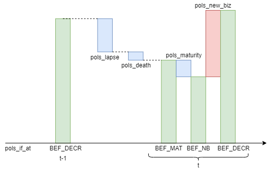
"BEF_DECR": Before lapse and death"BEF_MAT": Before maturity"BEF_NB": Before new business
The figure below illustrates how various policy inflows and outflows
are modeled in this model for one calculation step
from time t-1 to time t.
pols_lapse(t) and pols_death(t)
are the number of lapse and death from t-1 to t.
It is assumed that policies mature at the beginning of each month,
and new business policies enter at the beginning of the month
but after the maturity in that month.
Although the default model points are all new business policies,
CashValue_SE reads the duration of each model
point at time 0 from the model point file.
The duration of a model point being N months (N > 0) means
N months have elapsed before time 0 since the issue of the model point.
If the duration is -N months, the model point is issued
N months after time 0.
model_point_table has the duration_mth column,
and the column is read into the duration_mth(0).
If duration_mth(0) is positive,
the model point is in-force policies and
the number of policies
at time 0 is read from the policy_count column in model_point_table
into pols_if_init(), and
pols_if_at(0, "BEF_MAT") is set from pols_if_init().
duration_mth() increments by 1 each step. If duration_mth()
is negative, policy_count is read into pols_new_biz()
when duration_mth() becomes 0.
Account value roll-forward#
The account value per policy at each t is calculated
from the previous balance by adding cash inflows and
subtracting cash outflows.
The order and timing of the cashflows are as follows:
At the beginning of each month, premium net of loadings, if any, is put into the account value.
At the beginning of the month after the premium inflow, fees are deducted from the account value.
The investment income is earned on the account value throughout the month. Since policy decrement due to lapse and death is assumed to occur at the middle of the month, half the monthly investment return is assumed to be earned on the account values of the exiting policies.
Basic Usage#
Reading the model#
Create your copy of the savings library by following the steps on the Quick Start page. The model is saved as the folder named CashValue_SE in the copied folder.
To read the model from Spyder, right-click on the empty space in MxExplorer, and select Read Model. Click the folder icon on the dialog box and select the CashValue_SE folder.
Getting the results#
By default, the model has Cells
for outputting projection results as listed in the
Results section.
result_cf() outputs cashflows of the selected model point,
result_pv() outputs the present values of the cashflows,
result_pols() outputs the decrement table of the model point.
All the Cells outputs the results as pandas DataFrame.
See the Quick Start page for how to get the results in an MxConsole and view the results in MxDataViewer.
Changing the model point#
The model point to be selected is determined by
point_id in Projection.
It is 1 by default.
model_point_table contains 4 model points
as a pandas DataFrame.
To change the model point to another one, set the other model point’s ID
to point_id. Setting the new point_id clears
all the values of Cells that are specific to the previous model point.
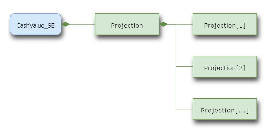
Getting multiple results#
The Projection space
is parameterized with point_id,
i.e. the Projection space can have dynamic child spaces, such as
Projection[1], Projection[2], Projection[3] …, each of which
represents the Projection for each of the model points.
Note
Getting results for too many dynamic child spaces
takes a considerable amount of time.
The default CashValue_SE model would take more than a minute
for 1000 model points on an ordinary spec PC.
To calculate for many model points,
consider using the CashValue_ME model.
Model Specifications#
The CashValue_SE model has only one UserSpace,
named Projection,
and all the Cells and References are defined in the space.
The Projection Space#
The main Space in the CashValue_SE model.
Projection is the only Space defined
in the CashValue_SE model, and it contains
all the logic and data used in the model.
Parameters and References
(In all the sample code below,
the global variable Projection refers to the
Projection Space.)
- point_id#
The ID of the selected model point.
point_idis defined as a Reference, and its value is used for determining the selected model point. By default,1is assigned. To select another model point, assign its model point ID to it:>>> Projection.point_id = 2
point_idis also defined as the parameter of theProjectionSpace, which makes it possible to create dynamic child space for multiple model points:>>> Projection.parameters ('point_id',) >>> Projection[1] <ItemSpace CashValue_SE.Projection[1]> >>> Projection[2] <ItemSpace CashValue_SE.Projection[2]>
See also
- model_point_table#
All model points as a DataFrame. By default, 4 model points are defined. The DataFrame has an index named
point_id, andmodel_point()returns a record as a Series whose index value matchespoint_id. The DataFrame has the following columns:spec_idage_at_entrysexpolicy_termpolicy_countsum_assuredduration_mthpremium_ppav_pp_init
Cells defined in
Projectionwith the same names as these columns return the corresponding column’s values for the selected model point.>>> Projection.model_poit_table spec_id age_at_entry sex ... premium_pp av_pp_init poind_id ... 1 A 20 M ... 500000 0 2 B 50 M ... 500000 0 3 C 20 M ... 1000 0 4 D 50 M ... 1000 0 [4 rows x 10 columns]
The DataFrame is saved in the Excel file model_point_samples.xlsx placed in the model folder.
model_point_tableis created by Projection’s new_pandas method, so that the DataFrame is saved in the separate file. The DataFrame has the injected attribute of_mx_dataclident:>>> Projection.model_point_table._mx_dataclient <PandasData path='model_point_table_samples.xlsx' filetype='excel'>
- disc_rate_ann#
Annual discount rates by duration as a pandas Series.
>>> Projection.disc_rate_ann
year
0      0.00000
1      0.00555
2      0.00684
3      0.00788
4      0.00866

146    0.03025
147    0.03033
148    0.03041
149    0.03049
150    0.03056
Name: disc_rate_ann, Length: 151, dtype: float64
The Series is saved in the Excel file disc_rate_ann.xlsx placed in the model folder.
disc_rate_annis created by Projection’s new_pandas method, so that the Series is saved in the separate file. The Series has the injected attribute of_mx_dataclident:>>> Projection.disc_rate_ann._mx_dataclient <PandasData path='disc_rate_ann.xlsx' filetype='excel'>
See also
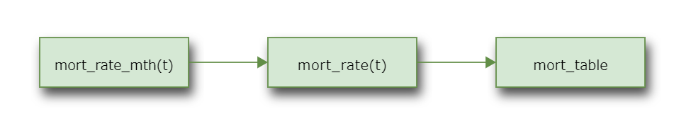
- mort_table#
Mortality table by age and duration as a DataFrame. See basic_term_sample.xlsx included in this library for how the sample mortality rates are created.
>>> Projection.mort_table
            0         1         2         3         4         5
Age
18   0.000231  0.000254  0.000280  0.000308  0.000338  0.000372
19   0.000235  0.000259  0.000285  0.000313  0.000345  0.000379
20   0.000240  0.000264  0.000290  0.000319  0.000351  0.000386
21   0.000245  0.000269  0.000296  0.000326  0.000359  0.000394
22   0.000250  0.000275  0.000303  0.000333  0.000367  0.000403
..        ...       ...       ...       ...       ...       ...
116  1.000000  1.000000  1.000000  1.000000  1.000000  1.000000
117  1.000000  1.000000  1.000000  1.000000  1.000000  1.000000
118  1.000000  1.000000  1.000000  1.000000  1.000000  1.000000
119  1.000000  1.000000  1.000000  1.000000  1.000000  1.000000
120  1.000000  1.000000  1.000000  1.000000  1.000000  1.000000

[103 rows x 6 columns]
The DataFrame is saved in the Excel file mort_table.xlsx placed in the model folder.
mort_tableis created by Projection’s new_pandas method, so that the DataFrame is saved in the separate file. The DataFrame has the injected attribute of_mx_dataclident:>>> Projection.mort_table._mx_dataclient <PandasData path='mort_table.xlsx' filetype='excel'>
See also
- std_norm_rand#
Random numbers drawn from the standard normal distribution.
A Series of random numbers drawn from the standard normal distribution indexed with
scen_idandt. Used for generating investment returns. Seeinv_return_table().
- scen_id#
Selected scenario ID
An integer indicating the selected scenario ID.
scen_idis referenced in byinv_return_mth()as one of the keys to select a scenario fromstd_norm_rand.
- surr_charge_table#
Surrender charge rates by duration.
A DataFrame of multiple patterns of surrender charge rates by duration. The column labels indicate
surr_charge_id(). By default,"type_1","type_2"and"type_3"are defined.
- product_spec_table#
Table of product specs.
A DataFrame of product spec parameters by
spec_id.model_point_tableandproduct_spec_tablecolumns are joined inmodel_point_table_ext(), and theproduct_spec_tablecolumns become part of the model point attributes. Theproduct_spec_tablecolumns are read by the Cells with the same names as the columns:>>> Projection.product_spec_table premium_type has_surr_charge surr_charge_id load_prem_rate is_wl spec_id A SINGLE False NaN 0.10 False B SINGLE True type_1 0.00 False C LEVEL False NaN 0.10 True D LEVEL True type_3 0.05 True
Projection parameters#
The time step of the model is monthly. Cashflows and other time-dependent
variables are indexed with t.
Projection is carried out separately for individual model points.
proj_len() calculates the number of months to be
projected for the selected model point.
Cashflows and other flows that accumulate throughout a period
indexed with t denote the sums of the flows from t til t+1.
Balance items indexed with t denote the amount at t.
|
Projection length in months |
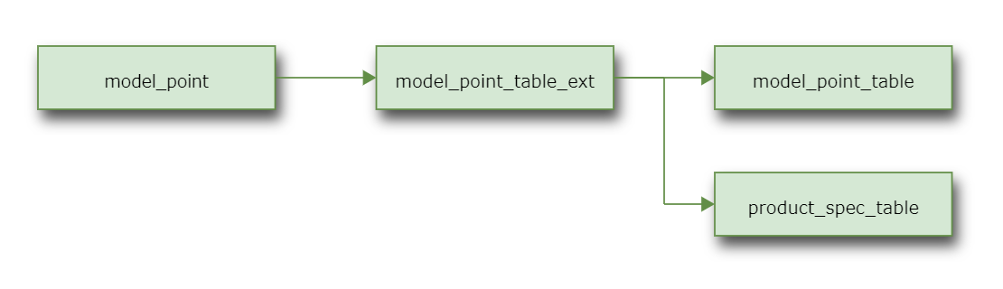
Model point data#
The model point data stored in an Excel file named model_point_table.xlsx
under the model folder is read into model_point_table.
Policy attributes that only vary by product spec are
stored separately in another Excel file named product_spec_table.xlsx,
and read into product_spec_table.
The product_spec_table attributes are joined with
model_point_table in model_point_table_ext()
and referenced from model_point().
The selected model point as a Series |
|
Extended model point table |
|
|
The sex of the selected model point |
The sum assured of the selected model point |
|
The policy term of the selected model point. |
|
|
The attained age at time t. |
The age at entry of the selected model point |
|
|
Duration of the selected model point at |
|
Duration of the selected model point at |
Whether surrender charge applies |
|
|
Whether the model point is whole life |
Rate of premium loading |
|
ID of surrender charge pattern |
|
Type of premium payment |
|
Initial account value per policy |
Assumptions#
The mortality table is stored in an Excel file named mort_table.xlsx
under the model folder, and is read into mort_table as a DataFrame.
mort_rate() looks up mort_table and picks up
the annual mortality rate to be applied for the selected
model point at time t.
mort_rate_mth() converts mort_rate() to the monthly mortality
rate to be applied during the month starting at time t.
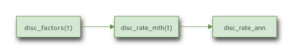
The discount rate data is stored in an Excel file named disc_rate_ann.xlsx
under the model folder, and is read into disc_rate_ann as a Series.
The lapse by duration is defined by a formula in lapse_rate().
expense_acq() holds the acquisition expense per policy at t=0.
expense_maint() holds the maintenance expense per policy per annum.
The maintenance expense inflates at a constant rate
of inflation given as inflation_rate().
The last age of mortality tables |
|
|
Mortality rate to be applied at time t |
Monthly mortality rate to be applied at time t |
|
Discount factors. |
|
Monthly discount rate |
|
|
Lapse rate |
Acquisition expense per policy |
|
Annual maintenance expense per policy |
|
The inflation factor at time t |
|
Inflation rate |
Policy values#
By default, the amount of death benefit for each policy (claim_pp())
is set equal to sum_assured.
premium_pp() is the single premium amount if the model point
represents single premium policies (i.e. premium_type() is "SINGLE"),
or the monthly premium amount if the model point represents
level premium policies (i.e. premium_type() is "LEVEL").
|
Claim per policy |
|
Premium amount per policy |
Maintenance fee per account value |
|
|
Cost of insurance rate per account value |
Surrender charge rate |
Policy decrement#
At t=0
If the selected model point represents in-force policies, i.e.
the duration_mth of the model point in model_point_table
is positive, pols_if_at(0, "BEF_MAT") is set to
the value through pols_if_init().
At each projection step
pols_if_at(t, timing) represents
the number of policies at t.
The timing parameter can take the following string values.
"BEF_MAT": Before maturity"BEF_NB": Before new business"BEF_DECR": Before lapse and death
Policy flows and in-force at each timing from t-1 to t
are calculated recursively as follows:
pols_if_at(t-1, "BEF_DECR")is calculated by addingpols_new_biz(t-1)topols_if_at(t-1, "BEF_NB").pols_if_at(t, "BEF_MAT")is calculated by deductingpols_lapse(t)andpols_death(t)frompols_if_at(t-1, "BEF_DECR").pols_if_at(t, "BEF_NB")is calculated by deductingpols_maturity(t)frompols_if_at(t, "BEF_MAT").pols_if_at(t, "BEF_DECR")is calculated bypols_new_biz(t)frompols_if_at(t, "BEF_NB").
It is assumed that policies mature at the beginning of each month,
and new business policies enter at the beginning of the month
but after the maturity in that month.
pols_if(t) is an alias
for pols_if_at(t, "BEF_MAT").
The figure below illustrates how various policy inflows and outflows
are modeled in this model for one calculation step
from time t-1 to time t.
|
Number of death |
|
Number of policies in-force |
|
Number of policies in-force |
Initial number of policies in-force |
|
|
Number of lapse |
Number of maturing policies |
|
|
Number of new business policies |
Account Value#
av_pp_at(t, timing) calculates the account value per policy
at t.
Since av_pp_at() can take multiple values for the same t
depending on the timing of various cashflows into and out of the
account value, the second parameter timing is used
to specify the timing of measuring the account value.
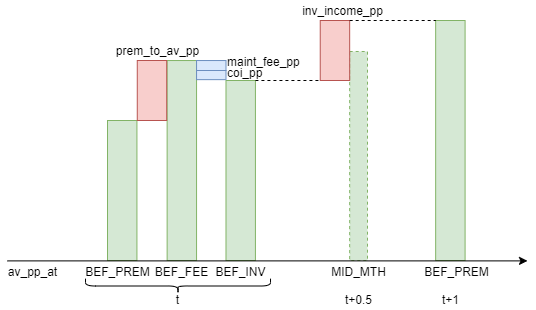
av_pp_at(t, 'BEF_PREM') indicates
the account value before premium payment for the month.
At time 0, it is read from av_pp_init(),
otherwise its calculated from the previous period
as av_pp_at(t-1, 'BEF_INV') plus
inv_income_(t-1).
av_pp_at(t, 'BEF_FEE') indicates
the account value after the premium payment before fee deduction, and
is calculated as av_pp_at(t, 'BEF_PREM') plus
prem_to_av_pp().
av_pp_at(t, 'BEF_INV') indicates
the account value after then fee deduction before earning investment yield, and
is calculated as av_pp_at(t, 'BEF_FEE') minus
maint_fee_pp() and coi_pp().
av_pp_at(t, 'MID_MTH') indicates
the account value at t+0.5, and half of inv_income()
is earned. av_pp_at(t, 'MID_MTH') is
for policies exiting by lapse and death during the month.
|
Investment income on account value |
Investment income on account value per policy |
|
Rate of investment return |
|
Table of investment return rates |
|
|
Account value per policy |
Net amount at risk per policy |
|
|
Cost of insurance charges per policy |
Per-policy premium portion put in the account value |
|
|
Maintenance fee per policy |
|
Account value in-force |
|
Premium portion put in account value |
|
Account value taken out to pay claim |
Claim in excess of account value |
|
|
Cost of insurance charges |
|
Maintenance fee deducted from account value |
|
Change in account value |
Check account value roll-forward |
Cashflows#
Cashflows are calculated as its per-policy amount times the number of policies.
The expense cashflow consists of acquisition expenses at issue and monthly maintenance expenses spent each month.
By default, commissions are defined as 5% premiums.
|
Surrender charge |
|
Claims |
|
Commissions |
|
Premium income |
|
Expenses |
|
Net cashflow |
Margin Analysis#
net_cf() can be expressed as the sum of expense and mortality
margins. The expense margin is defined as the sum of
premium loading, surrender charge and maintenance fees
net of commissions and expenses.
The mortality margin is defined coi() net of claims_over_av().
Expense margin |
|
Mortality margin |
|
Check consistency between net cashflow and margins |
Present values#
The Cells whose names start with pv_ are for calculating
the present values of the cashflows indicated by the rest of their names.
pv_pols_if() is not used
in CashValue_SE and BasicTerm_ME.
|
Present value of claims |
Present value of commissions |
|
Present value of expenses |
|
Present value of net cashflows. |
|
Present value of policies in-force |
|
Present value of premiums |
|
Present value of change in account value |
|
Present value of investment income |
|
Check present value summation |
Results#
result_cf() outputs the cashflows of the selected model point
as a DataFrame:
>>> result_cf()
       Premiums        Death  ...  Change in AV  Net Cashflow
0    50000000.0   999.844857  ...  4.447174e+07  2.033342e+06
1           0.0   991.084783  ... -1.065060e+06  3.292919e+04
2           0.0   982.401460  ...  2.039757e+05  3.208843e+04
3           0.0   973.794216  ... -2.527055e+05  3.228511e+04
4           0.0   965.262383  ... -7.053975e+05  3.210189e+04
..          ...          ...  ...           ...           ...
116         0.0  1346.032341  ...  2.851405e+04  2.368209e+04
117         0.0  1343.713636  ... -2.927039e+05  2.370171e+04
118         0.0  1341.398924  ...  4.096877e+05  2.347573e+04
119         0.0  1339.088201  ...  4.207922e+05  2.381819e+04
120         0.0     0.000000  ... -3.263268e+07  0.000000e+00

[121 rows x 9 columns]
result_pv() outputs the present values of the cashflows:
>>> result_pv()
      Premiums          Death  ...  Commissions  Net Cashflow
PV  50000000.0  135032.740399  ...    2500000.0  4.957050e+06
Result table of cashflows |
|
Result table of present value of cashflows |
|
Result table of policy decrement |
Cells Descriptions#
- proj_len()[source]#
Projection length in months
proj_len()indicates how many months the projection for the selected model point should be carried out. Defined as:12 * policy_term() - duration_mth(0) + 1
See also
- model_point()[source]#
The selected model point as a Series
model_point()looks upmodel_point_table_ext(), and returns as a Series the row whose index is the value ofpoint_id.Example
In the code below
Projectionrefers to theProjectionspace:>>> Projection.point_id 1 >>> Projection.model_point() spec_id A age_at_entry 20 sex M policy_term 10 policy_count 100 sum_assured 500000 duration_mth 0 premium_pp 500000 av_pp_init 0 premium_type SINGLE has_surr_charge False surr_charge_id NaN load_prem_rate 0.1 is_wl False Name: 1, dtype: object >>> Projection.point_id = 2 >>> Projection.model_point() spec_id C age_at_entry 20 sex M policy_term 9999 policy_count 100 sum_assured 500000 duration_mth 0 premium_pp 1000 av_pp_init 0 premium_type LEVEL has_surr_charge False surr_charge_id NaN load_prem_rate 0.1 is_wl True Name: 3, dtype: object
See also
- model_point_table_ext()[source]#
Extended model point table
Returns an extended
model_point_tableby joiningproduct_spec_tableon thespec_idcolumn.See also
- sex()[source]#
The sex of the selected model point
Note
This cells is not used by default.
The element labeled
sexof the Series returned bymodel_point().
- sum_assured()[source]#
The sum assured of the selected model point
The element labeled
sum_assuredof the Series returned bymodel_point().
- policy_term()[source]#
The policy term of the selected model point.
The element labeled
policy_termof the Series returned bymodel_point().
- age_at_entry()[source]#
The age at entry of the selected model point
The element labeled
age_at_entryof the Series returned bymodel_point().
- duration_mth(t)[source]#
Duration of the selected model point at
tin monthsIndicates how many months the policies have been in-force at
t. The initial value at time 0 is read from theduration_mthcolumn inmodel_point_tablethroughmodel_point(). Increments by 1 astincrements. Negative values ofduration_mth()indicate future new business policies. For example, If theduration_mth()is -15 at time 0, the model point is issued att=15.See also
- has_surr_charge()[source]#
Whether surrender charge applies
Trueif surrender charge on account value applies upon lapse,Falseif other wise. By default, the value is read from thehas_surr_chargecolumn inmodel_point().See also
- is_wl()[source]#
Whether the model point is whole life
Trueif the model point is whole life,Falseif other wise. By default, the value is read from theis_wlcolumn inmodel_point(). This attribute is used to determinpolicy_term(). IfTrue,policy_term()is defined asmort_table_last_age()minusage_at_entry(). IfFalse,policy_term()is read frommodel_point().See also
- load_prem_rate()[source]#
Rate of premium loading
This rate times
premium_pp()is collected from each premium and the rest is added to the account value.By default, the value is read from the
load_prem_ratecolumn inmodel_point().See also
- surr_charge_id()[source]#
ID of surrender charge pattern
A string to indicate the ID of the surrender charge pattern. The ID should be one of the column names in
surr_charge_tableifhas_surr_charge()isTrue.See also
Type of premium payment
Returns a string indicating the payment type, which is either
"LEVEL"if level payment, or"SINGLE"if single payment.
- av_pp_init()[source]#
Initial account value per policy
For existing business at time
0, returns initial per-policy accout value read from theav_pp_initcolumn inmodel_point(). For new business, 0 should be entered in the column.See also
- mort_table_last_age()[source]#
The last age of mortality tables
Returns the last age whose mortality rates are all 1. If no such age is found, return the last index of the tables
See also
- disc_factors()[source]#
Discount factors.
Vector of the discount factors as a Numpy array. Used for calculating the present values of cashflows.
See also
- disc_rate_mth()[source]#
Monthly discount rate
Nummpy array of monthly discount rates from time 0 to
proj_len()- 1 defined as:(1 + disc_rate_ann)**(1/12) - 1
See also
- lapse_rate(t)[source]#
Lapse rate
By default, the lapse rate assumption is defined by duration as:
max(0.1 - 0.02 * duration(t), 0.02)
See also
- inflation_rate()[source]#
Inflation rate
The inflation rate to be applied to the expense assumption. By defualt it is set to
0.01.See also
- claim_pp(t, kind)[source]#
Claim per policy
The claim amount per policy. The second parameter is to indicate the type of the claim, and it takes a string, which is either
"DEATH","LAPSE"or"MATURITY".The death benefit as denoted by
"DEATH", is the greater ofsum_assured()and mid-month account value (av_pp_at(t, "MID_MTH")).The surrender benefit as denoted by
"LAPSE"and the maturity benefit as denoted by"MATURITY"are equal to the mid-month account value.See also
Premium amount per policy
Single premium amount if
premium_type()is"SINGLE", monthly premium amount ifpremium_type()is"LEVEL".
- maint_fee_rate()[source]#
Maintenance fee per account value
The rate of maintenance fee on account value each month. Set to
0.01 / 12by default.See also
- coi_rate(t)[source]#
Cost of insurance rate per account value
The cost of insuranc rate per account value per month. By default, it is set to 1.1 times the monthly mortality rate.
See also
- surr_charge_rate(t)[source]#
Surrender charge rate
Surrender charge rate to be applied for lapsed policies
- pols_if(t)[source]#
Number of policies in-force
pols_if(t)is an alias forpols_if_at(t, "BEF_MAT").See also
- pols_if_at(t, timing)[source]#
Number of policies in-force
pols_if_at(t, timing)calculates the number of policies in-force at timet. The second parametertimingtakes a string value to indicate the timing of in-force, which is either"BEF_MAT","BEF_NB"or"BEF_DECR".BEF_MAT
The number of policies in-force before maturity after lapse and death. At time 0, the value is read from
pols_if_init(). For time > 0, defined as:pols_if_at(t-1, "BEF_DECR") - pols_lapse(t-1) - pols_death(t-1)
BEF_NB
The number of policies in-force before new business after maturity. Defined as:
pols_if_at(t, "BEF_MAT") - pols_maturity(t)
BEF_DECR
The number of policies in-force before lapse and death after new business. Defined as:
pols_if_at(t, "BEF_NB") + pols_new_biz(t)
- pols_if_init()[source]#
Initial number of policies in-force
Number of in-force policies at time 0 referenced from
pols_if_at(0, "BEF_MAT").
- pols_lapse(t)[source]#
Number of lapse
Number of policies decreased by lapse during
tandt+1.See also
- pols_maturity(t)[source]#
Number of maturing policies
The policy maturity occurs when
duration_mth()equals 12 timespolicy_term(). The amount is equal topols_if_at(t, "BEF_MAT").otherwise
0.
- pols_new_biz(t)[source]#
Number of new business policies
The number of new business policies. The value
duration_mth(0)for the selected model point is read from thepolicy_countcolumn inmodel_point(). If the value is 0 or negative, the model point is new business at t=0 or at t whenduration_mth(t)is 0, and thepols_new_biz(t)is read from thepolicy_countinmodel_point().See also
- inv_income(t)[source]#
Investment income on account value
Investment income earned on account value during each period. For the plicies decreased by lapse and death, half the investment income is credited.
- inv_income_pp(t)[source]#
Investment income on account value per policy
Investment income on account value defined as:
inv_return_mth(t) * av_pp_at(t, "BEF_INV")
See also
- inv_return_mth(t)[source]#
Rate of investment return
Rate of monthly investment return for
scen_idandtread frominv_return_table()See also
- inv_return_table()[source]#
Table of investment return rates
Returns a Series of monthly investment retuns. The Series is indexed with
scen_idandtwhich is inherited fromstd_norm_rand.\[\exp\left(\left(\mu-\frac{\sigma^{2}}{2}\right)\Delta{t}+\sigma\sqrt{\Delta{t}}\epsilon\right)-1\]where \(\mu=2\%\), \(\sigma=3\%\), \(\Delta{t}=\frac{1}{12}\), and \(\epsilon\) is a randome number from the standard normal distribution.
See also
- av_pp_at(t, timing)[source]#
Account value per policy
av_at(t, timing)calculates the total amount of account value at timetfor the policies represented by a model point.At each
t, the events that change the account value balance occur in the following order:Premium payment
Fee deduction
Investment income is assumed to be earned throughout each month, so at the middle of the month when death and lapse occur, half the investment income for the month is credited.
The second parameter
timingtakes a string to indicate the timing of the account value, which is either"BEF_PREM","BEF_FEE","BEF_INV"or"MID_MTH".BEF_PREM
Account value before premium payment. At the start of the projection (i.e. when
t=0), the account value is set toav_pp_init().BEF_FEE
Account value after premium payment before fee deduction
BEF_INV
Account value after fee deduction before crediting investemnt return
MID_MTH
Account value at middle of month (
t+0.5) when half the investment retun for the month is credited
- net_amt_at_risk(t)[source]#
Net amount at risk per policy
Return sum assured net of account value per policy.
See also
- coi_pp(t)[source]#
Cost of insurance charges per policy
The cost of insurance charges per policy. Defined as the coi charge rate times net amount at risk per policy.
See also
- prem_to_av_pp(t)[source]#
Per-policy premium portion put in the account value
The amount of premium per policy net of loading, which is put in the accoutn value.
See also
- av_at(t, timing)[source]#
Account value in-force
av_at(t, timing)calculates the total amount of account value at timetfor the policies represented by a model point.At each
t, the events that change the account value balance occur in the following order:Maturity
New business and premium payment
Fee deduction
The second parameter
timingtakes a string to indicate the timing of the account value, which is either"BEF_MAT","BEF_NB"or"BEF_FEE".BEF_MAT
The amount of account value before maturity, defined as:
av_pp_at(t, "BEF_PREM") * pols_if_at(t, "BEF_MAT")
BEF_NB
The amount of account value before new business after maturity, defined as:
av_pp_at(t, "BEF_PREM") * pols_if_at(t, "BEF_NB")
BEF_FEE
The amount of account value before lapse and death after new business, defined as:
av_pp_at(t, "BEF_FEE") * pols_if_at(t, "BEF_DECR")
See also
- prem_to_av(t)[source]#
Premium portion put in account value
The amount of premiums net of loadings, which is put in the accoutn value.
See also
- claims_from_av(t, kind)[source]#
Account value taken out to pay claim
The part of the claim amount that is paid from account value. The second parameter takes a string indicating the type of the claim, which is either
"DEATH","LAPSE"or"MATURITY".Death benefit is denoted by
"DEATH", is defined as:av_pp_at(t, "MID_MTH") * pols_death(t)
When the account value is greater than the death benefit, the death benefit equates to the account value.
Surrender benefit as denoted by
"LAPSE"is defined as:av_pp_at(t, "MID_MTH") * pols_lapse(t)
As the surrender benefit is defined as account value less surrender charge, when there is no surrender charge the surrender benefit equates to the account value.
Maturity benefit as denoted by
"MATURITY"is defined as:av_pp_at(t, "BEF_PREM") * pols_maturity(t)
By default, the maturity benefit equates to the account value of maturing policies.
- claims_over_av(t)[source]#
Claim in excess of account value
The amount of death benefits in excess of account value.
coi()net of this amount represents mortality margin.See also
- coi(t)[source]#
Cost of insurance charges
The cost of insurance charges deducted from acccount values each period.
See also
- av_change(t)[source]#
Change in account value
Change in account value during each period, defined as:
av_at(t+1, 'BEF_MAT') - av_at(t, 'BEF_MAT')
See also
- check_av_roll_fwd()[source]#
Check account value roll-forward
Returns
Tureifav_at(t+1, "BEF_NB")equates to the following expression for allt, otherwise returnsFalse:av_at(t, "BEF_NB") + prem_to_av(t) - maint_fee(t) - coi(t) + inv_income(t) - claims_from_av(t, "DEATH") - claims_from_av(t, "LAPSE") - claims_from_av(t, "MATURITY"))
- surr_charge(t)[source]#
Surrender charge
Surrender charge rate times account values of lapsed policies
- claims(t, kind=None)[source]#
Claims
The claim amount during the period from
ttot+1. The optional second parameter is for indicating the type of the claim, and it takes a string, which is either"DEATH","LAPSE"or"MATURITY", or defaults toNoneto indicate the total of all the types of claims during the period.The death benefit as denoted by
"DEATH"is defined as:claim_pp(t) * pols_death(t)
The surrender benefit as denoted by
"LAPSE"is defined as:claims_from_av(t, "LAPSE") - surr_charge(t)
The maturity benefit as denoted by
"MATURITY"is defined as:claims_from_av(t, "MATURITY")
Premium income
Premium income during the period from
ttot+1defined as:premium_pp() * pols_if_at(t, "BEF_DECR")
See also
- expenses(t)[source]#
Expenses
Expenses during the period from
ttot+1defined as the sum of acquisition expenses and maintenance expenses. The acquisition expenses are modeled asexpense_acq()timespols_new_biz(). The maintenance expenses are modeled asexpense_maint()timesinflation_factor()timespols_if_at()before decrement.
- net_cf(t)[source]#
Net cashflow
Net cashflow for the period from
ttot+1defined as:premiums(t) + inv_income(t) - claims(t) - expenses(t) - commissions(t) - av_change(t)
- margin_expense(t)[source]#
Expense margin
Expense margin is defined as the sum of premium loading, surrender charge and maintenance fees net of commissions and expenses.
The sum of the expense margin and mortality margin add up to the net cashflow.
- margin_mortality(t)[source]#
Mortality margin
Mortality margin is defined
coi()net ofclaims_over_av().The sum of the expense margin and mortality margin add up to the net cashflow.
See also
- check_margin()[source]#
Check consistency between net cashflow and margins
Returns
Trueifnet_cf()equates to the sum ofmargin_expense()andmargin_mortality()for allt, otherwise, returnsFalse.See also
- pv_net_cf()[source]#
Present value of net cashflows.
Defined as:
pv_premiums() + pv_inv_income()
- pv_claims() - pv_expenses() - pv_commissions() - pv_av_change()
- pv_pols_if()[source]#
Present value of policies in-force
Note
This cells is not used by default.
The discounted sum of the number of in-force policies at each month. It is used as the annuity factor for calculating
net_premium_pp().
Present value of premiums
See also
- pv_inv_income()[source]#
Present value of investment income
The discounted sum of monthly investment income.
See also
- check_pv_net_cf()[source]#
Check present value summation
Check if the present value of
net_cf()matches the sum of the present values each cashflows. Returns the check result asTrueorFalse.See also