TVOG of a maturity guarantee under G2++ scenarios#
CashValue_ME_G2PP is lifelib’s savings model CashValue_ME_EX4 with its economic inputs taken from the space ESG, a copy of BasicG2PP’s G2PP space. ESG reads g2pp_input.xlsx in the library folder. Its scenario 0 is the certainty-equivalent (CE) scenario, which follows the initial forward curve, so one run gives both terms of
TVOG = mean of the present values over the stochastic scenarios − the present value in the CE scenario.
This notebook shows the model points, the TVOG of the guaranteed minimum accumulation benefit (GMAB) on the delivered input, how it depends on the bond fund the account value is invested in, and how the Monte Carlo results compare with the closed form.
Click the badge below to run this notebook online on Google Colab. You need a Google account and need to be logged in to it to run this notebook on Google Colab. 
The next code cell below is relevant only when you run this notebook on Google Colab. It installs lifelib and creates a copy of the library for this notebook.
[1]:
import sys, os

if 'google.colab' in sys.modules:
    lib = 'economic'; lib_dir = '/content/'+ lib
    if not os.path.exists(lib_dir):
        !pip install lifelib
        import lifelib; lifelib.create(lib, lib_dir)

    %cd $lib_dir
[2]:
import matplotlib.pyplot as plt
import modelx as mx
import numpy as np
import pandas as pd
from matplotlib.ticker import PercentFormatter
from modelx.core.errors import FormulaError
from scipy import stats

model = mx.read_model("CashValue_ME_G2PP")
proj, esg = model.Projection, model.ESG
T = 120                                   # every model point matures in month 120
n_scen = len(esg.scen_index())
print(f"{n_scen - 1:,} stochastic scenarios plus the CE scenario; fund {esg.fund_id()}")
1,000 stochastic scenarios plus the CE scenario; fund BOND_MIX
[3]:
# Chart style: light-mode tokens of the reference palette, one categorical slot per fund
SURFACE, INK, INK_2, MUTED = "#fcfcfb", "#0b0b0b", "#52514e", "#898781"
GRID, AXIS = "#e1e0d9", "#c3c2b7"
FUND_COLORS = {"CASH": "#2a78d6", "BOND_MIX": "#1baf7a", "BOND_10Y": "#eb6834"}
plt.rcParams.update({
    "figure.facecolor": SURFACE, "axes.facecolor": SURFACE, "savefig.facecolor": SURFACE,
    "axes.edgecolor": AXIS, "axes.linewidth": 1, "axes.grid": True, "grid.color": GRID,
    "grid.linewidth": 1, "axes.spines.top": False, "axes.spines.right": False,
    "axes.labelcolor": INK_2, "axes.titlecolor": INK, "axes.titlesize": 11,
    "axes.titlelocation": "left", "xtick.color": AXIS, "ytick.color": AXIS,
    "xtick.labelcolor": INK_2, "ytick.labelcolor": INK_2, "legend.frameon": False,
    "legend.labelcolor": INK_2, "lines.linewidth": 2, "lines.solid_capstyle": "round",
    "figure.dpi": 110, "font.size": 9.5,
})
Model points#
All nine model points are 10-year policies: 100 policies with a sum assured of 500,000 each. Points 1, 2, 5, 6 and 9 pay a single premium. For them, the account value after the premium, AV0, divided by the present value of the sum assured, SA · P(0, 10), shows how far the guarantee is in the money: below 1 it pays in the CE scenario. Points 3, 4, 7 and 8 pay level premiums every month, build up account values far above the sum assured, and their GMAB costs nothing.
[4]:
mps = proj.model_point_table_ext()
sa = (proj.sum_assured() * proj.pols_maturity(T))[::n_scen]
av0 = proj.av_at(0, "BEF_FEE")[::n_scen]
is_single = (mps["premium_type"] == "SINGLE").to_numpy()
points = pd.DataFrame({
    "premium type": mps["premium_type"], "premium per policy": mps["premium_pp"], "SA": sa,
    "AV0": np.where(is_single, av0, np.nan),
    "AV0 / (SA P(0,10))": np.where(is_single, av0 / (sa * esg.mkt_zcb(T)), np.nan).round(3),
}, index=mps.index)
single = points.index[is_single].tolist()
points
[4]:
| premium type | premium per policy | SA | AV0 | AV0 / (SA P(0,10)) | |
|---|---|---|---|---|---|
| point_id | |||||
| 1 | SINGLE | 500000 | 50000000.0 | 50000000.0 | 1.267 |
| 2 | SINGLE | 475000 | 50000000.0 | 47500000.0 | 1.203 |
| 3 | LEVEL | 450000 | 50000000.0 | NaN | NaN |
| 4 | LEVEL | 425000 | 50000000.0 | NaN | NaN |
| 5 | SINGLE | 400000 | 50000000.0 | 40000000.0 | 1.013 |
| 6 | SINGLE | 375000 | 50000000.0 | 37500000.0 | 0.950 |
| 7 | LEVEL | 350000 | 50000000.0 | NaN | NaN |
| 8 | LEVEL | 325000 | 50000000.0 | NaN | NaN |
| 9 | SINGLE | 300000 | 50000000.0 | 30000000.0 | 0.760 |
TVOG on the delivered input#
result_tvog() gives, for each model point, the present value in the CE scenario, the mean over the stochastic scenarios, their difference (the TVOG) and the standard error of the mean from antithetic pairs. For the GMAB cost:
[5]:
tvog = proj.result_tvog()
tvog["GMAB"].round(0)
[5]:
| CE | mean | TVOG | SE | |
|---|---|---|---|---|
| point_id | ||||
| 1 | 0.0 | 0.0 | 0.0 | 0.0 |
| 2 | 0.0 | 618.0 | 618.0 | 453.0 |
| 3 | 0.0 | 0.0 | 0.0 | 0.0 |
| 4 | 0.0 | 0.0 | 0.0 | 0.0 |
| 5 | 0.0 | 771177.0 | 771177.0 | 31328.0 |
| 6 | 1970018.0 | 2255066.0 | 285048.0 | 21916.0 |
| 7 | 0.0 | 0.0 | 0.0 | 0.0 |
| 8 | 0.0 | 0.0 | 0.0 | 0.0 |
| 9 | 9470018.0 | 9467934.0 | -2084.0 | 10635.0 |
The GMDB costs nothing because EX4 has no mortality. The TVOG of the present value of net cash flows is the GMAB’s TVOG with the opposite sign, plus Monte Carlo noise. Premium loads, commissions and expenses are fixed amounts, and their mean deflated value equals their CE value only up to sampling error. The noise is largest for the level-premium points 3 and 7, whose premiums carry 10% loads; on the delivered input it is within one standard error:
[6]:
pd.DataFrame({"GMAB TVOG": tvog["GMAB"]["TVOG"],
              "net cash flow TVOG": tvog["net cash flow"]["TVOG"],
              "sum (noise)": tvog["GMAB"]["TVOG"] + tvog["net cash flow"]["TVOG"],
              "net cash flow SE": tvog["net cash flow"]["SE"]}).round(0)
[6]:
| GMAB TVOG | net cash flow TVOG | sum (noise) | net cash flow SE | |
|---|---|---|---|---|
| point_id | ||||
| 1 | 0.0 | -34.0 | -34.0 | 45.0 |
| 2 | 618.0 | -652.0 | -34.0 | 456.0 |
| 3 | 0.0 | 16900.0 | 16900.0 | 22170.0 |
| 4 | 0.0 | -34.0 | -34.0 | 45.0 |
| 5 | 771177.0 | -771211.0 | -34.0 | 31330.0 |
| 6 | 285048.0 | -285082.0 | -34.0 | 21924.0 |
| 7 | 0.0 | 13137.0 | 13137.0 | 17234.0 |
| 8 | 0.0 | -34.0 | -34.0 | 45.0 |
| 9 | -2084.0 | 2050.0 | -34.0 | 10661.0 |
TVOG by fund#
The ESG takes the fund from fund_id in the workbook. To compare funds without editing the workbook, the next cell overrides the value of ESG’s fund_id cell (esg.fund_id[()] = ...), which recalculates everything that depends on it, and restores the workbook’s value at the end with esg.fund_id.clear_all().
For an all-cash fund and for a fund holding a single maturity, formula_gmab_g2pp(t) gives the exact GMAB cost, from the variance s² of the log growth of the account value. A mix of maturities has no exact closed form.
[7]:
funds = ["CASH", "BOND_MIX", "BOND_10Y"]
p_T = esg.mkt_zcb(T)
results = {}
for fund in funds:
    esg.fund_id[()] = fund
    gmab = proj.result_tvog()["GMAB"].loc[single]
    try:
        formula, s2 = proj.formula_gmab_g2pp(T), esg.fund_logvar(T)
    except FormulaError:
        formula, s2 = pd.Series(np.nan, index=single), np.nan
    results[fund] = {"gmab": gmab, "formula": formula, "s2": s2}
esg.fund_id.clear_all()
print(f"fund restored to {esg.fund_id()}")
for fund in funds:
    s2 = results[fund]["s2"]
    note = f"{np.sqrt(s2 / 10):.2%} a year" if s2 == s2 else "no closed form"
    print(f"{fund:9s} volatility of the account value's log growth over 10 years: {note}")
fund restored to BOND_MIX
CASH      volatility of the account value's log growth over 10 years: 3.39% a year
BOND_MIX  volatility of the account value's log growth over 10 years: no closed form
BOND_10Y  volatility of the account value's log growth over 10 years: 3.31% a year
[8]:
moneyness = points.loc[single, "AV0 / (SA P(0,10))"].to_numpy()
unit = (sa * p_T)[[p - 1 for p in single]]           # SA P(0,10) of each point
grid = np.linspace(0.7, 1.32, 200)


def closed_form_tvog(r, s2):
    """TVOG per unit of SA P(0,T) at moneyness r = AV0 / (SA P(0,T))."""
    s = np.sqrt(s2)
    d1 = (-np.log(r) + s2 / 2) / s
    return stats.norm.cdf(d1) - r * stats.norm.cdf(d1 - s) - np.maximum(1 - r, 0)


fig, axes = plt.subplots(1, len(funds), figsize=(11, 3.9), sharex=True, sharey=True)
for ax, fund in zip(axes, funds):
    color, res = FUND_COLORS[fund], results[fund]
    gmab = res["gmab"]
    if res["s2"] == res["s2"]:
        ax.plot(grid, closed_form_tvog(grid, res["s2"]), color=color)
    else:
        ax.text(0.97, 0.95, "no closed form for\na mix of maturities", transform=ax.transAxes,
                ha="right", va="top", color=INK_2)
    ax.errorbar(moneyness, gmab["TVOG"] / unit, yerr=1.96 * gmab["SE"] / unit, fmt="o",
                color=color, markersize=7, markeredgecolor=SURFACE, markeredgewidth=2,
                elinewidth=1.5, capsize=0, zorder=3)
    ax.axhline(0, color=AXIS, linewidth=1)
    ax.set_title(fund)
    ax.set_xlabel("AV0 / (SA × P(0, 10))")
    ax.yaxis.set_major_formatter(PercentFormatter(1.0, decimals=1))
axes[0].set_ylabel("TVOG / (SA × P(0, 10))")
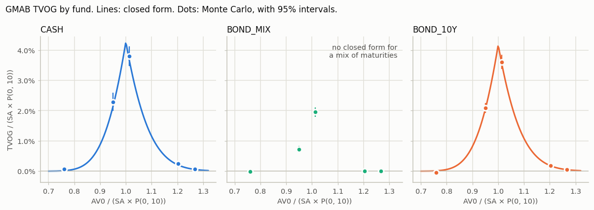
fig.suptitle("GMAB TVOG by fund. Lines: closed form. Dots: Monte Carlo, with 95% intervals.",
             x=0.01, ha="left", color=INK, fontsize=11)
fig.tight_layout()
plt.show()
[9]:
table = pd.concat({fund: pd.DataFrame({
    "TVOG": results[fund]["gmab"]["TVOG"],
    "SE": results[fund]["gmab"]["SE"],
    "closed-form TVOG": results[fund]["formula"] - results[fund]["gmab"]["CE"],
}) for fund in funds}, axis=1)
table.round(0)
[9]:
| CASH | BOND_MIX | BOND_10Y | |||||||
|---|---|---|---|---|---|---|---|---|---|
| TVOG | SE | closed-form TVOG | TVOG | SE | closed-form TVOG | TVOG | SE | closed-form TVOG | |
| 1 | 30139.0 | 11152.0 | 22775.0 | 0.0 | 0.0 | NaN | 20830.0 | 7190.0 | 19166.0 |
| 2 | 95945.0 | 19976.0 | 79078.0 | 618.0 | 453.0 | NaN | 74277.0 | 13677.0 | 69855.0 |
| 5 | 1499775.0 | 66074.0 | 1445854.0 | 771177.0 | 31328.0 | NaN | 1423709.0 | 46774.0 | 1407136.0 |
| 6 | 903679.0 | 61062.0 | 843310.0 | 285048.0 | 21916.0 | NaN | 820980.0 | 32955.0 | 809690.0 |
| 9 | 24362.0 | 18318.0 | 6112.0 | -2084.0 | 10635.0 | NaN | -18990.0 | 21597.0 | 4931.0 |
The closed form runs through the Monte Carlo results for the all-cash fund and the 10-year bond fund, within their sampling error. Those two curves are almost the same: over ten years, holding 10-year zero-coupon bonds and rolling them every month makes the account value about as volatile as holding cash. The mixed fund, 20% cash, 30% 5-year and 50% 10-year bonds, makes the guarantee much cheaper. Its value falls less when rates rise, and higher reinvestment returns afterwards make up for the fall, so the account value at maturity is less uncertain.
The library’s test suite checks these results more tightly: in every scenario the GMAB cost equals D(T) · (SA − AV0 · fund growth)⁺ recomputed from the ESG paths, to 1e-10 of the sum assured (tests/test_cashvalue_me_g2pp.py).