The IntegratedLife Model#
Overview#
The IntegratedLife model is a comprehensive and practical projection
tool designed for real-world actuarial tasks.
In practical actuarial applications, actuaries need to run projections for multiple products with varying parameters, assumptions, and scenarios. These projections often involve different model point sets at various base dates.
The IntegratedLife model allows you to define multiple runs to address these needs.
Each run has its own run_id,
enabling you to associate specific assumption files, economic scenarios,
and model point files with each run_id.
Runs are represented in the model as ItemSpaces within the Run space,
such as Run[1], Run[2], and so on.
IntegratedLife also supports a mechanism to
define logic and data by products.
In the Run space,
spaces are defined by inheriting from ProductBase.
These are called product spaces.
A product space represents the logic and data for a specific family of products.
At the moment, only one product space, GMXB
is defined, but more product spaces will be added in future releases.
You can define parameters specific to each user space.
Model Structure#
In IntegratedLife, following spaces are defined.
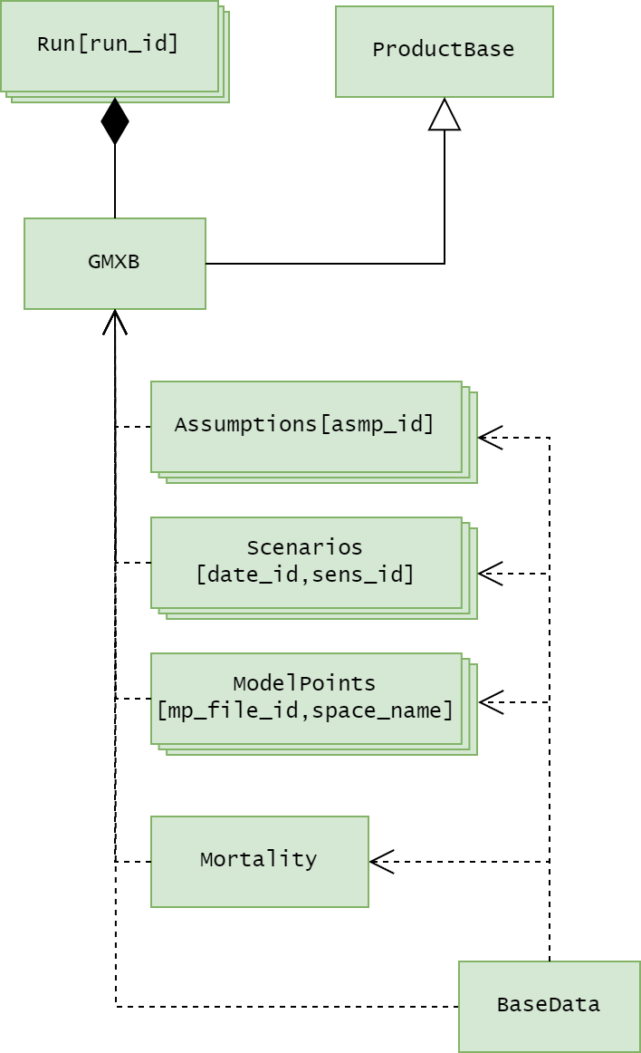
BaseData: Reads model parameters from the parameter fileMortality: Reads mortality tables from the mortality fileModelPoints: Reads model point data from model point filesScenarios: Reads economic data from filesAssumptions: Reads assumption data from filesProductBase: Serves as the base space for specific product spaces defined in runsRun: Represents projection runsGMXB: The Product space for GMAB and GMDB policies
The diagram below depicts the relationships between the spaces.

The BaseData space reads parameters from a parameter file.
BaseData is referenced in many other spaces,
and its parameters are used universally in the model.
BaseData also reads surrender charge tables,
which are static in the model.
See the Parameter File section and the BaseData page
for how the parameters are defined in the parameter file.
The Mortality space reads mortality tables from a mortality file.
The file path of the mortality file is defined by the table_dir and mort_file parameters
in the parameter file. See the Mortality page for more details.
The Run space is parameterized with run_id, and is the base space for individual runs.
Each individual run is a dynamic item space of the Run space with a specific
run_id value, such as Run[1], Run[2], and so on.
The Run space has product spaces
that are derived from the ProductBase space.
Currently, only one product space, GMXB is defined.
All the logic and names in GMXB
are actually defined in ProductBase,
and nothing is redefined or added in GMXB.
Depending on the value of run_id,
different values for run parameters are read from the parameter file.
The run parameters include, asmp_id and mp_file_id, which are used to determine
what assumption file and model point file should be used for the run.
The Assumptions space is parameterized with
asmp_id.
As explained above, asmp_id is a run parameter,
and is defined in the RunParams sheet
in the parameter file as a string ID that identifies
a set of assumptions to be used for a specific run.
The assumption file whose name ends with
asmp_id is used for the run.
The ModelPoints space is parameterized with
mp_file_id and
space_name.
mp_file_id is a run parameter,
and is defined in the RunParams sheet
in the parameter file as a string ID.
The model point file whose name ends with mp_file_id
and space_name is selected for the run.
The Scenarios space is parameterized
with date_id and
sens_id.
date_id is a run parameter
defined in the RunParams sheet,
sens_id
is defined as sens_int_rate in RunParams in the parameter file.
date_id is used to identify the interest rate file,
while sens_id
is used to identify what sheet should be used in the selected file.
Input Files#
Parameter File#
By default, the IntegratedLife model reads model parameters
from a parameter file in BaseData.
The parameter file is an excel file named “model_parameters.xlsx” by default,
and located in the same directory as the model is located.
The name of the parameter file is specified by
parameter_file in the model.
In the parameter file, parameters are defined in the following sheets, depending on how their values should vary by.
CostParamsRunParamsSpaceParamsSheets with product space names (Only “GMXB” by default)
The ConstParams sheet defines constant parameters,
whose values are constant over all runs across all products.
The RunParams sheet defines run parameters, whose values vary by runs.
The SpaceParams sheet defines space parameters,
whose values vary by product spaces.
The same parameter can be defined in more than one sheets of the three,
but it must not appear more than once in the same sheet.
The ParamList sheet is for listing all the parameters defined in the three sheets,
and its read_from column indicates from what sheet the value of each parameter should be defined.
However, the following basic parameters should be constant parameters:
table_dirspec_tablesasmp_file_prefixmodel_point_dirmp_file_prefixmort_filescen_dirscen_param_filescen_file_prefix
For some basic parameters, the read_from values cannot be changed.
See BaseData for the complete list of these
parameters.
Parameters defined in these three sheets are called fixed parameters,
because their values do not vary by model points within each product space.
All the fixed parameters in a product space are combined in
fixed_params() as a Series.
The sheets with the names of product spaces are per-space sheets.
by default, only one per-space sheet, GMXB is defined.
A par-space sheet is specific to the product space that its name represents.
For example, the GMXB sheet defines parameters specific to the GMXB space.
Parameters in a par-space sheet is indexed by the two left most columns,
product_id and plan_id.
The parameters are appended to model point data by looking up product_id and plan_id in
model_point_table_ext().
Model Point Files#
By default, sample model point files are stored in
the model_point_data folder in the library.
Model point files are prepared by user space.
The file name is constructed using a prefix,
mp_file_id and
space_name,
all concatenated by underscores, followed by “.csv”.
See ModelPoints for more details.
Assumption Files#
Assumption files are Excel files containing assumption data.
Assumption files are identified by asmp_id, and associated to
runs through a run parameter, asmp_id.
By default, assumption files are stored in
the input_tables folder in the library.
The file name is constructed using a prefix, “assumptions” and
asmp_id
concatenated by underscores, followed by “.xlsx”.
See Assumptions for more details.
Product Spec File#
A product spec file is an Excel file containing parameters related
to product specs that do not vary by projection dates.
By default, the file is named “product_spec_tables.xlsx”,
and located in the input_tables folder in the library.
The name and location of the file are specified
by the constant parameters, spec_tables and table_dir,
in the parameter file.
Currently, only a surrender charge table is defined.
Mortality Table File#
By default, the mortality table file is named “mortality_tables.xlsx”,
and located in the input_tables folder in the library.
The name and location of the file are specified
by the constant parameters, mort_file and table_dir,
in the parameter file.
See Mortality for more details.
Economic Data File#
By default, files for economic data are located in the economic_data folder in the library.
By default, risk free rates are used for discounting and interest rate assumptions.
Risk free rates at a certain date, identified by date_id
are contained in an Excel file, named “risk_free_YYYYMM.xlsx”,
where “YYYYMM” is the date_id.
The name and location of the interest rate files
Each risk-free rate file has 3 sheets, “BASE”, “UP” and “DOWN”. The sheet name is used as a key when determining interest rate sensitivity.
See Scenarios for more details.
Basic Usage#
Reading the model#
Create your copy of the appliedlife library by following the steps on the Quick Start page. The model is saved as the folder named IntegratedLife in the copied folder.
To read the model from Spyder with the modelx plug-in, right-click on the empty space in MxExplorer, and select Read Model. Click the folder icon on the dialog box and select the IntegratedLife folder.
To read the model on IPython console, use the read_model function in modelx.
>>> import modelx as mx

>>> m = mx.read_model("IntegratedLife")
Running the results#
To run the model, simply execute result Cells,
such as result_pv(),
of a product space, such as GMXB,
in a dynamic subspace of Run,
such as Run[1],
where the number in [] is a specific run_id.
>>> m.Run(1).GMXB.result_pv()

                 Premiums         Death  ...  Change in AV  Net Cashflow
point_id scen                            ...
1        1     50000000.0  4.535395e+06  ...  1.141797e+07  6.097680e+06
         2     50000000.0  4.592794e+06  ...  1.244402e+07  6.732840e+06
         3     50000000.0  4.514334e+06  ...  1.215701e+07  6.499784e+06
         4     50000000.0  4.667772e+06  ...  1.250695e+07  6.648902e+06
         5     50000000.0  4.403177e+06  ...  1.138434e+07  6.107113e+06
                  ...           ...  ...           ...           ...
8        96    32500000.0  3.013149e+06  ...  5.651292e+06 -1.669267e+07
         97    32500000.0  3.050556e+06  ...  8.690729e+06 -6.839240e+05
         98    32500000.0  3.013149e+06  ...  3.701018e+06 -1.436214e+07
         99    32500000.0  3.230455e+06  ...  8.484874e+06  1.174996e+06
         100   32500000.0  3.013149e+06  ...  7.439794e+06 -1.503688e+06

[800 rows x 9 columns]


>>> m.Run(1).GMXB.result_cf()

         Premiums        Claims      Expenses   Commissions  Net Cashflow
0    3.300000e+10  6.885792e+07  4.033333e+08  1.280000e+09  4.305433e+08
1    0.000000e+00  6.887329e+07  3.328038e+06  0.000000e+00  2.310506e+07
2    0.000000e+00  6.875446e+07  3.322756e+06  0.000000e+00  2.313363e+07
3    0.000000e+00  6.868379e+07  3.317490e+06  0.000000e+00  2.311497e+07
4    0.000000e+00  6.869832e+07  3.312239e+06  0.000000e+00  2.318471e+07
..            ...           ...           ...           ...           ...
116  0.000000e+00  2.288671e+08  1.870365e+06  0.000000e+00  7.103725e+06
117  0.000000e+00  2.264772e+08  1.851697e+06  0.000000e+00  7.054587e+06
118  0.000000e+00  2.238152e+08  1.833222e+06  0.000000e+00  6.974249e+06
119  0.000000e+00  2.216954e+08  1.814959e+06  0.000000e+00  6.897696e+06
120  0.000000e+00  2.076927e+10  0.000000e+00  0.000000e+00 -2.087250e+09

[121 rows x 5 columns]

>>> m.Run(1).GMXB.result_pols()

          pols_if  pols_maturity  pols_new_biz  pols_death  pols_lapse
0        0.000000       0.000000         80000   15.888508  177.398389
1    79806.713103       0.000000             0   15.849889  176.849853
2    79614.013360       0.000000             0   15.811388  176.251368
3    79421.950604       0.000000             0   15.773013  175.675413
4    79230.502178       0.000000             0   15.734762  175.131998
..            ...            ...           ...         ...         ...
116  40772.225418       0.000000             0   90.248214  350.153733
117  40331.823472       0.000000             0   89.268431  346.231945
118  39896.323096       0.000000             0   88.299619  341.906948
119  39466.116529       0.000000             0   87.342607  337.606448
120  39041.167475   39041.167475             0    0.000000    0.000000

[121 rows x 5 columns]
result_sample() returns
the detailed result for a single model point on a single scenario.
Alternatively, excel_sample()
opens Excel and output the sample result on an Excel workbook.
>>> m.Run(1).GMXB.excel_sample()

       premiums     inv_income  ...  inv_return_mth  disc_rate_mth
0    50000000.0   36668.209367  ...        0.000816       0.003883
1           0.0 -832902.827593  ...       -0.018567       0.003883
2           0.0  136715.311689  ...        0.003113       0.003883
3           0.0   15294.022885  ...        0.000348       0.003883
4           0.0  125878.367168  ...        0.002869       0.003883
..          ...            ...  ...             ...            ...
116         0.0 -223430.982443  ...       -0.007303       0.002830
117         0.0  640062.777645  ...        0.021289       0.002830
118         0.0   62510.277083  ...        0.002057       0.002830
119         0.0 -427654.831703  ...       -0.014189       0.002830
120         0.0       0.000000  ...        0.014783       0.002837

[121 rows x 38 columns]
