The BasicTerm_ME Model#
Overview#
The BasicTerm_ME model is a faster reimplementation of
the BasicTerm_SE model.
The BasicTerm_ME model reproduces the same results as
BasicTerm_SE much faster.
Each formula to be applied to all the model points
operates on the entire set of model points at once
with the help of Numpy and Pandas.
The default product specs, assumptions and input data
are the same as BasicTerm_SE.
Changes from BasicTerm_M#
Below is the list of
Cells and References that are newly added or updated from BasicTerm_M.
premium_table<new>duration_mth<new>pols_if_at()<new>pols_new_biz()<new>result_pols()<new>
In summary, below are the main changes
common to BasicTerm_ME and BasicTerm_SE.
Refer to the descritpion for BasicTerm_SE for
more details.
model_point_tablehas theduration_mthcolumn, to indicate the duration of the model point at time 0,pols_if_at(t, timing)is introduced to allow multiple values for the number of policy in-force at the same time at different policy flow timing.premium_tableholds premium rate data calculated outside the model.
Speed comparison#
The main advantage of the BasicTerm_ME model over the
BasicTerm_SE model is its speed.
Below is the result of a simple speed comparison between the two models.
The machine used for this comparison is a consumer PC equipped
with Intel Core i5-6500T CPU and 16GB RAM.
>>> timeit.timeit("[Projection[i].pv_net_cf() for i in range(1, 101)]", globals=globals(), number=1)
5.971486999999996
>>> timeit.timeit("pv_net_cf()", globals=globals(), number=1)
3.9130262000000045
Note that only the first 100 model points were run with BasicTerm_SE
while all the 10000 model points were run with BasicTerm_ME.
While BasicTerm_SE took about 6.0 seconds for the 100 model points,
BasicTerm_ME took only 3.9 seconds for the 10000 model points.
This means BasicTerm_ME
runs about 153 times faster than BasicTerm_SE.
The run time of BasicTerm_SE
is shorter that BasicTerm_S because
the projection length of each model point is shorter for
BasicTerm_SE.
Formula examples#
Most formulas in the BasicTerm_ME model
are the same as those in BasicTerm_SE.
However, some formulas are updated since they cannot
be applied to vector operations without change.
For example, below shows how
pols_maturity, the number of maturing policies
at time t, is defined differently in
BasicTerm_SE and in
BasicTerm_ME.
def pols_maturity(t):
    if duration_mth(t) == policy_term() * 12:
        return pols_if_at(t, "BEF_MAT")
    else:
        return 0
 def pols_maturity(t):
     return (duration_mth(t) == policy_term() * 12) * pols_if_at(t, "BEF_MAT")
In BasicTerm_SE,
policy_term() returns an integer,
such as 10 indicating a policy term of the selected model point in years,
so the if clause checks if the value of duration_mth()
is equal to the policy term in month:
>>> policy_term()
10

>>> pols_maturity(120)
0.6534679117893804
In contrast, policy_term() in BasicTerm_ME returns
a Series of policy terms of all the model points.
If the if clause were
defined in the same way as in the BasicTerm_SE,
it would result in an error,
because the condition duration_mth(t) == policy_term() * 12 for a certain t
returns a Series of boolean values and it is ambiguous
for the Series to be in the if condition.
Further more, whether the if branch or the else branch should
be evaluated needs to be determined element-wise,
but the if statement would not allow such element-wise branching.
Instead of using the if statement, the formula in BasicTerm_ME
achieves the element-wise conditional operation by multiplication
by a Series of boolean values.
In the formula in BasicTerm_ME,
pols_if_at(t, "BEF_MAT")
returns the numbers of policies at time t for all the model points
as a Series.
Multiplying it
by (duration_mth(t) == policy_term() * 12) replaces
the numbers of policies with 0 for model points whose policy terms in month
are not equal to t. This operation is effectively an element-wise if
operation:
>>> policy_term()
point_id
1        10
2        20
3        10
4        20
5        15
         ..
9996     20
9997     15
9998     20
9999     20
10000    15
Name: policy_term, Length: 10000, dtype: int64


>>> (duration_mth(119) == policy_term() * 12)
policy_id
1         True
2        False
3        False
4        False
5        False

9996     False
9997     False
9998     False
9999     False
10000    False
Length: 10000, dtype: bool


>>> pols_maturity(119)
policy_id
1        56.696979
2         0.000000
3         0.000000
4         0.000000
5         0.000000

9996      0.000000
9997      0.000000
9998      0.000000
9999      0.000000
10000     0.000000
Length: 10000, dtype: float64
Since projections for in-force policies do not start from their issuance,
the premium rates are calculated externaly by
BasicTerm_M and fed into the model as a table.
The premium rates are stored in premium_table.xlsx in the model folder
and read into premium_table as a Series.
Basic Usage#
Reading the model#
Create your copy of the basiclife library by following
the steps on the Quick Start page.
The model is saved as the folder named BasicTerm_ME in the copied folder.
To read the model from Spyder, right-click on the empty space in MxExplorer,
and select Read Model.
Click the folder icon on the dialog box and select the
BasicTerm_ME folder.
Getting the results#
By default, the model has Cells
for outputting projection results as listed in the
Results section.
result_cf() outputs total cashflows of all the model points,
and result_pv() outputs the present values of the cashflows
by model points.
Both Cells outputs the results as pandas DataFrame.
By following the same steps explained in the Quick Start page using this model, You can get the results in an MxConsole and show the results as tables in MxDataViewer.
Changing the model point#
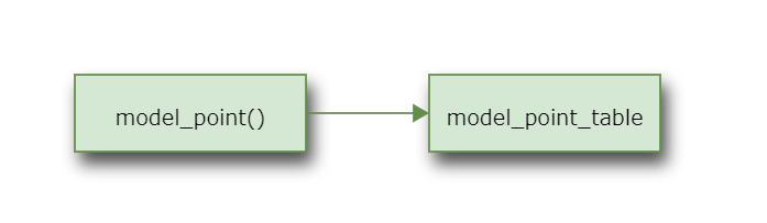
By default, model_point() returns the entire model_point_table:
>>> Projection.model_point.formula
def model_point():
    return model_point_table
The calculations in Projection apply to all the model points
in model_point_table.
To limit the calculation target, change the model_point() formula
so that model_point() returns a DataFrame that contains
only the target rows.
For example, to select only the model point 1:
>>> Projection.model_point.formula
def model_point():
    return model_point_table.loc[1:1]
There are many methods of DataFrame for selecting its rows. See the pandas documentation for details.
When selecting only one model point, make sure that model_point()
returns the model point as a DataFrame not as a Series.
In the code example above, model_point_table.loc[1:1]
is specified instead of model_point_table.loc[1],
because model_point_table.loc[1] would return the model point as a Series.
Also, you should be careful not to accidentally update the original DataFrame
held as model_point_table.
Model Specifications#
The BasicTerm_ME model has only one UserSpace,
named Projection,
and all the Cells and References are defined in the space.
The Projection Space#
The main Space in the BasicTerm_ME model.
Projection is the only Space defined
in the BasicTerm_ME model, and it contains
all the logic and data used in the model.
Parameters and References
(In all the sample code below,
the global variable Projection refers to the
Projection Space.)
- model_point_table#
All model points as a DataFrame. The sample model point data was generated by generate_model_points_with_duration.ipynb included in the library. By default,
model_point()returns this entiremodel_point_table. The DataFrame has an index namedpoint_id, and has the following columns:age_at_entrysexpolicy_termpolicy_countsum_assuredduration_mth
Cells defined in
Projectionwith the same names as these columns return the corresponding columns.>>> Projection.model_poit_table age_at_entry sex ... sum_assured duration_mth policy_id ... 1 47 M ... 622000 1 2 29 M ... 752000 210 3 51 F ... 799000 15 4 32 F ... 422000 125 5 28 M ... 605000 55 ... .. ... ... ... 9996 47 M ... 827000 157 9997 30 M ... 826000 168 9998 45 F ... 783000 146 9999 39 M ... 302000 11 10000 22 F ... 576000 166 [10000 rows x 6 columns]
The DataFrame is saved in the Excel file model_point_table.xlsx placed in the model folder.
model_point_tableis created by Projection’s new_pandas method, so that the DataFrame is saved in the separate file. The DataFrame has the injected attribute of_mx_dataclident:>>> Projection.model_point_table._mx_dataclient <PandasData path='model_point_table.xlsx' filetype='excel'>
Premium rate table by entry age and duration as a Series. The table is created using
BasicTerm_Mas demonstrated in create_premium_table.ipynb. The table is stored in premium_table.xlsx in the model folder.>>> Projection.premium_table age_at_entry policy_term 20 10 0.000046 15 0.000052 20 0.000057 21 10 0.000048 15 0.000054 ... 58 15 0.000433 20 0.000557 59 10 0.000362 15 0.000471 20 0.000609 Name: premium_rate, Length: 120, dtype: float64
- disc_rate_ann#
Annual discount rates by duration as a pandas Series.
>>> Projection.disc_rate_ann
year
0      0.00000
1      0.00555
2      0.00684
3      0.00788
4      0.00866

146    0.03025
147    0.03033
148    0.03041
149    0.03049
150    0.03056
Name: disc_rate_ann, Length: 151, dtype: float64
The Series is saved in the Excel file disc_rate_ann.xlsx placed in the model folder.
disc_rate_annis created by Projection’s new_pandas method, so that the Series is saved in the separate file. The Series has the injected attribute of_mx_dataclident:>>> Projection.disc_rate_ann._mx_dataclient <PandasData path='disc_rate_ann.xlsx' filetype='excel'>
See also
- mort_table#
Mortality table by age and duration as a DataFrame. See basic_term_sample.xlsx included in this library for how the sample mortality rates are created.
>>> Projection.mort_table
            0         1         2         3         4         5
Age
18   0.000231  0.000254  0.000280  0.000308  0.000338  0.000372
19   0.000235  0.000259  0.000285  0.000313  0.000345  0.000379
20   0.000240  0.000264  0.000290  0.000319  0.000351  0.000386
21   0.000245  0.000269  0.000296  0.000326  0.000359  0.000394
22   0.000250  0.000275  0.000303  0.000333  0.000367  0.000403
..        ...       ...       ...       ...       ...       ...
116  1.000000  1.000000  1.000000  1.000000  1.000000  1.000000
117  1.000000  1.000000  1.000000  1.000000  1.000000  1.000000
118  1.000000  1.000000  1.000000  1.000000  1.000000  1.000000
119  1.000000  1.000000  1.000000  1.000000  1.000000  1.000000
120  1.000000  1.000000  1.000000  1.000000  1.000000  1.000000

[103 rows x 6 columns]
The DataFrame is saved in the Excel file mort_table.xlsx placed in the model folder.
mort_tableis created by Projection’s new_pandas method, so that the DataFrame is saved in the separate file. The DataFrame has the injected attribute of_mx_dataclident:>>> Projection.mort_table._mx_dataclient <PandasData path='mort_table.xlsx' filetype='excel'>
See also
Projection parameters#
This is a new business model and all model points are issued at time 0.
The time step of the model is monthly. Cashflows and other time-dependent
variables are indexed with t.
Cashflows and other flows that accumulate throughout a period
indexed with t denotes the sums of the flows from t til t+1.
Balance items indexed with t denotes the amount at t.
|
Projection length in months |
The max of all projection lengths |
Model point data#
The model point data is stored in an Excel file named model_point_table.xlsx under the model folder.
Target model points |
|
|
The sex of the model points |
The sum assured of the model points |
|
The policy term of the model points. |
|
|
The attained age at time t. |
The age at entry of the model points |
|
|
Duration of model points at |
|
Duration of model points at |
Assumptions#
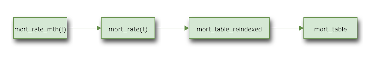
The mortality table is stored in an Excel file named mort_table.xlsx
under the model folder, and is read into mort_table as a DataFrame.
mort_table_reindexed() returns a mortality table
reshaped from mort_table, which is a Series
indexed with Age and Duration.
mort_rate() looks up mort_table_reindexed() and picks up
the annual mortality rates to be applied for all the
model points at time t and returns them in a Series.
mort_rate_mth() converts mort_rate() to the monthly mortality
rate to be applied during the month starting at time t.
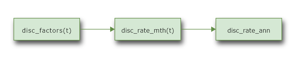
The discount rate data is stored in an Excel file named disc_rate_ann.xlsx
under the model folder, and is read into disc_rate_ann as a Series.
The lapse by duration is defined by a formula in lapse_rate().
expense_acq() holds the acquisition expense per policy at t=0.
expense_maint() holds the maintenance expense per policy per annum.
The maintenance expense inflates at a constant rate
of inflation given as inflation_rate().
|
Mortality rate to be applied at time t |
Monthly mortality rate to be applied at time t |
|
MultiIndexed mortality table |
|
Discount factors. |
|
Monthly discount rate |
|
|
Lapse rate |
Acquisition expense per policy |
|
Annual maintenance expense per policy |
|
The inflation factor at time t |
|
Inflation rate |
Policy values#
By default, the amount of death benefit for each policy (claim_pp())
is set equal to sum_assured.
The payment method is monthly whole term payment for all model points.
The monthly premium per policy (premium_pp())
is calculated for each policy
as (1 + loading_prem()) times net_premium_pp().
The net premium is calculated so that the present value of the
net premiums equates to the present values of claims.
This product is assumed to have no surrender value.
|
Claim per policy |
Net premium per policy |
|
Loading per premium |
|
Monthly premium per policy |
Policy decrement#
The initial number of policies is set to 1 per model point by default, and decreases through out the policy term by lapse and death. At the end of the policy term the remaining number of policies mature.
|
Number of death occurring at time t |
|
Number of policies in-force |
|
Number of policies in-force |
Initial number of policies in-force |
|
|
Number of lapse occurring at time t |
Number of maturing policies |
|
|
Number of new business policies |
Cashflows#
An acquisition expense at t=0 and maintenance expenses thereafter comprise expense cashflows.
Commissions are assumed to be paid out during the first year and the commission amount is assumed to be 100% premium during the first year and 0 afterwards.
|
Claims |
|
Commissions |
|
Premium income |
|
Expenses |
|
Net cashflow |
Present values#
The Cells whose names start with pv_ are for calculating
the present values of the cashflows indicated by the rest of their names.
pols_if() is not a cashflow, but used as annuity factors
in calculating net_premium_pp().
Present value of claims |
|
Present value of commissions |
|
Present value of expenses |
|
Present value of net cashflows. |
|
Present value of policies in-force |
|
Present value of premiums |
Results#
result_cf() outputs the total cashflows of all the model points
as a DataFrame:
>>> result_cf()
         Premiums        Claims      Expenses   Commissions  Net Cashflow
0    3.481375e+07  2.551366e+07  2.722470e+06  2.304871e+06  4.272750e+06
1    3.458612e+07  2.533530e+07  2.777227e+06  2.271010e+06  4.202583e+06
2    3.460642e+07  2.532024e+07  2.992697e+06  2.316894e+06  3.976592e+06
3    3.446821e+07  2.526094e+07  2.816155e+06  2.308385e+06  4.082731e+06
4    3.440382e+07  2.527465e+07  2.896164e+06  2.319160e+06  3.913840e+06
..            ...           ...           ...           ...           ...
272  1.509838e+05  2.281406e+05  8.909740e+03  0.000000e+00 -8.606662e+04
273  1.292070e+05  1.969228e+05  6.464827e+03  0.000000e+00 -7.418061e+04
274  9.360930e+04  1.447365e+05  4.187218e+03  0.000000e+00 -5.531445e+04
275  5.851123e+04  9.225161e+04  1.942107e+03  0.000000e+00 -3.568248e+04
276  0.000000e+00  0.000000e+00  0.000000e+00  0.000000e+00  0.000000e+00

[277 rows x 5 columns]
result_pv() outputs the present values of the cashflows by model points:
>>> result_pv()
            PV Premiums      PV Claims  ...  PV Commissions  PV Net Cashflow
policy_id                               ...
1          7.083791e+05  474803.297001  ...    85874.887301    108798.061916
2          9.950994e+04  109613.723658  ...        0.000000    -18305.709146
3          1.104613e+06  802437.653322  ...        0.000000    266073.249126
4          2.839117e+05  264723.616424  ...        0.000000    -18224.092562
5          4.399130e+05  352234.521794  ...        0.000000     32214.118896
                ...            ...  ...             ...              ...
9996       3.574210e+05  405869.354038  ...        0.000000    -58052.929127
9997       5.917467e+04   59908.482977  ...        0.000000     -5547.111546
9998       1.314719e+05  141951.671002  ...        0.000000    -14790.802910
9999       5.615703e+04   39215.159798  ...      372.420000      9219.186564
10000      7.927437e+03    7433.441293  ...        0.000000      -752.642292

[10000 rows x 5 columns]
Result table of cashflows |
|
Result table of present value of cashflows |
|
Result table of policy decrement |
Cells Descriptions#
- proj_len()[source]#
Projection length in months
proj_len()returns how many months the projection for each model point should be carried out for all the model point. Defined as:np.maximum(12 * policy_term() - duration_mth(0) + 1, 0)
Since this model carries out projections for all the model points simultaneously, the projections are actually carried out from 0 to
max_proj_lenfor all the model points.See also
- max_proj_len()#
The max of all projection lengths
Defined as
max(proj_len())See also
- model_point()[source]#
Target model points
Returns as a DataFrame the model points to be in the scope of calculation. By default, this Cells returns the entire
model_point_tablewithout change. To select model points, change this formula so that this Cells returns a DataFrame that contains only the selected model points.Examples
To select only the model point 1:
def model_point():
    return model_point_table.loc[1:1]
To select model points whose ages at entry are 40 or greater:
def model_point():
    return model_point_table[model_point_table["age_at_entry"] >= 40]
Note that the shape of the returned DataFrame must be the same as the original DataFrame, i.e.
model_point_table.When selecting only one model point, make sure the returned object is a DataFrame, not a Series, as seen in the example above where
model_point_table.loc[1:1]is specified instead ofmodel_point_table.loc[1].Be careful not to accidentally change the original table.
- sex()[source]#
The sex of the model points
Note
This cells is not used by default.
The
sexcolumn of the DataFrame returned bymodel_point().
- sum_assured()[source]#
The sum assured of the model points
The
sum_assuredcolumn of the DataFrame returned bymodel_point().
- policy_term()[source]#
The policy term of the model points.
The
policy_termcolumn of the DataFrame returned bymodel_point().
- age_at_entry()[source]#
The age at entry of the model points
The
age_at_entrycolumn of the DataFrame returned bymodel_point().
- duration_mth(t)[source]#
Duration of model points at
tin monthsIndicates how many months the policies have been in-force at
t. The initial values at time 0 are read from theduration_mthcolumn inmodel_point_tablethroughmodel_point(). Increments by 1 astincrements. Negative values ofduration_mth()indicate future new business policies. For example, If theduration_mth()is -15 at time 0, the model point is issued att=15.See also
- mort_rate(t)[source]#
Mortality rate to be applied at time t
Returns a Series of the mortality rates to be applied at time t. The index of the Series is
point_id, copied frommodel_point().
- mort_table_reindexed()[source]#
MultiIndexed mortality table
Returns a Series of mortlity rates reshaped from
mort_table. The returned Series is indexed by age and duration capped at 5.
- disc_factors()[source]#
Discount factors.
Vector of the discount factors as a Numpy array. Used for calculating the present values of cashflows.
See also
- disc_rate_mth()[source]#
Monthly discount rate
Nummpy array of monthly discount rates from time 0 to
max_proj_len()- 1 defined as:(1 + disc_rate_ann)**(1/12) - 1
See also
- lapse_rate(t)[source]#
Lapse rate
By default, the lapse rate assumption is defined by duration as:
max(0.1 - 0.02 * duration(t), 0.02)
See also
- claim_pp(t)[source]#
Claim per policy
The claim amount per plicy. Defaults to
sum_assured().
Net premium per policy
Note
This cells is not used by default.
The net premium per policy is defined so that the present value of net premiums equates to the present value of claims:
pv_claims() / pv_pols_if()
See also
- loading_prem()[source]#
Loading per premium
Note
This cells is not used by default.
0.5by default.See also
Monthly premium per policy
A Series of monthly premiums per policy for all the model points, calculated as:
np.around(sum_assured() * prem_rates, 2)
where the
prem_ratesis a Series of premium rates retrieved frompremium_table.
- pols_if(t)[source]#
Number of policies in-force
pols_if(t)is an alias forpols_if_at(t, "BEF_MAT").See also
- pols_if_at(t, timing)[source]#
Number of policies in-force
pols_if_at(t, timing)calculates the number of policies in-force at timet. The second parametertimingtakes a string value to indicate the timing of in-force, which is either"BEF_MAT","BEF_NB"or"BEF_DECR".BEF_MAT
The number of policies in-force before maturity after lapse and death. At time 0, the value is read from
pols_if_init(). For time > 0, defined as:pols_if_at(t-1, "BEF_DECR") - pols_lapse(t-1) - pols_death(t-1)
BEF_NB
The number of policies in-force before new business after maturity. Defined as:
pols_if_at(t, "BEF_MAT") - pols_maturity(t)
BEF_DECR
The number of policies in-force before lapse and death after new business. Defined as:
pols_if_at(t, "BEF_NB") + pols_new_biz(t)
- pols_if_init()[source]#
Initial number of policies in-force
Number of in-force policies at time 0 referenced from
pols_if_at(0, "BEF_MAT").
- pols_maturity(t)[source]#
Number of maturing policies
The policy maturity occurs when
duration_mth()equals 12 timespolicy_term(). The amount is equal topols_if_at(t, "BEF_MAT").otherwise
0.
- pols_new_biz(t)[source]#
Number of new business policies
The number of new business policies. The value
duration_mth(0)for the selected model point is read from thepolicy_countcolumn inmodel_point(). If the value is 0 or negative, the model point is new business at t=0 or at t whenduration_mth(t)is 0, and thepols_new_biz(t)is read from thepolicy_countinmodel_point().See also
- claims(t)[source]#
Claims
Claims during the period from
ttot+1defined as:claim_pp(t) * pols_death(t)
See also
- commissions(t)[source]#
Commissions
By default, 100% premiums for the first year, 0 otherwise.
See also
Premium income
Premium income during the period from
ttot+1defined as:premium_pp() * pols_if_at(t, "BEF_DECR")
See also
- expenses(t)[source]#
Expenses
Expenses during the period from
ttot+1defined as the sum of acquisition expenses and maintenance expenses. The acquisition expenses are modeled asexpense_acq()timespols_new_biz(). The maintenance expenses are modeled asexpense_maint()timesinflation_factor()timespols_if_at()before decrement.
- net_cf(t)[source]#
Net cashflow
Net cashflow for the period from
ttot+1defined as:premiums(t) - claims(t) - expenses(t) - commissions(t)
See also
- pv_net_cf()[source]#
Present value of net cashflows.
Defined as:
pv_premiums() - pv_claims() - pv_expenses() - pv_commissions()
- pv_pols_if()[source]#
Present value of policies in-force
Note
This cells is not used by default.
The discounted sum of the number of in-force policies at each month. It is used as the annuity factor for calculating
net_premium_pp().
Present value of premiums
See also