The CashValue_ME Model#
Overview#
The CashValue_ME model is a faster reimplementation of
the CashValue_SE model.
The CashValue_ME model reproduces the same results as
CashValue_SE, but is more suitable for
processing a large number of model points.
Each formula to be applied to all the model points
operates on the entire set of model points at once
with the help of Numpy and Pandas.
The default product specs, assumptions and input data
are the same as CashValue_SE.
Changes from CashValue_SE#
Below is the list of
Cells and References that are newly added or
updated from CashValue_SE.
max_proj_len<new>mort_table_reindexed()<new>
Running with 10000 model points#
The main advantage of the CashValue_ME model over the
CashValue_SE model is its speed.
By default, CashValue_ME is configured
to run the same 4 model points as the ones in CashValue_SE,
but a larger table of 10000 model points is also included in the model.
The larger model point table is saved in the model folder
as an Excel file named model_point_10000.xlsx,
and this table is read into the model as
a DataFrame named model_point_10000.
The 10000 model points are all new business at time 0, and
created by modifying the sample model points in basiclife.
To run the model with the larger model point table,
assign the table to model_point_table:
>>> Projection.model_point_table = Projection.model_point_10000
In the code above, Projection must be defined beforehand to
refer to the Projection space.
Below is the speed result of running the entire 10000 model points on a consumer PC equipped with Intel Core i5-6500T CPU and 16GB RAM.
>>> timeit.timeit("Projection.result_pv()", globals=globals(), number=1)
34.3045132

>>> Projection.result_pv()
               Premiums         Death  ...  Change in AV  Net Cashflow
policy_id                              ...
1          5.349200e+07  4.852612e+05  ...  4.465141e+06  1.881696e+06
2          4.446054e+07  1.356468e+07  ...  1.604824e+07  1.177058e+07
3          1.210841e+08  7.179706e+07  ...  2.796228e+07  2.192224e+07
4          3.038400e+07  2.938897e+05  ...  4.840159e+06  4.346383e+06
5          5.989500e+07  3.342985e+05  ...  7.238519e+06  7.671440e+06
                ...           ...  ...           ...           ...
9996       2.067500e+07  5.335816e+05  ...  3.627718e+06  1.951471e+06
9997       6.690600e+07  4.291283e+05  ...  8.984202e+06  4.590207e+06
9998       7.629662e+06  4.007463e+06  ...  1.982635e+06  1.441142e+06
9999       2.835552e+06  1.258307e+06  ...  8.583928e+05  4.917449e+05
10000      1.513202e+07  3.834462e+06  ...  6.555234e+06  3.667102e+06

[10000 rows x 9 columns]
The above run projects all model points for the max length of the entire model points:
>>> Projection.max_proj_len()
1141
Since product A and B are limited term up to 20 years
and C and D are whole life,
it may be more efficient to run the limited term and whole life model
points separately,
because the limited term model points don’t need as long the length
of projection period as C and D model points.
You can do so by defining, for example, seg_id to
filter model points in the formula of model_point().
The code below is an example of the modified formula of model_point()
to filter the model points by seg_id:
>>> Projection.model_point.formula
def model_point():
    """"Target model points
    ...
    """
    cond = model_point_table_ext()['is_wl'] == (True if seg_id == 'WL' else False)
    return model_point_table_ext().loc[cond]
Assigning "WL" to seg_id results in running only whole life model points,
while assigning anything other than "WL" results in running
limited term model points:
>>> Projection.seg_id = 'WL'

>>> timeit.timeit("Projection.result_pv()", globals=globals(), number=1)
24.311953799999998

>>> Projection.result_pv()
               Premiums         Death  ...  Change in AV  Net Cashflow
policy_id                              ...
2          4.446054e+07  1.356468e+07  ...  1.604824e+07  1.177058e+07
3          1.210841e+08  7.179706e+07  ...  2.796228e+07  2.192224e+07
6          5.051520e+06  3.011482e+06  ...  1.152065e+06  4.933033e+04
9          5.537287e+07  3.686858e+07  ...  1.126645e+07  7.784990e+06
10         2.957650e+07  1.156441e+07  ...  9.877157e+06  6.451814e+06
                ...           ...  ...           ...           ...
9988       5.051377e+05  1.692807e+05  ...  1.715821e+05  1.065215e+05
9989       2.889266e+07  1.769398e+07  ...  5.681889e+06  4.869589e+06
9998       7.629662e+06  4.007463e+06  ...  1.982635e+06  1.441142e+06
9999       2.835552e+06  1.258307e+06  ...  8.583928e+05  4.917449e+05
10000      1.513202e+07  3.834462e+06  ...  6.555234e+06  3.667102e+06

[5015 rows x 9 columns]

>>> Projection.max_proj_len()
1141

>>> Projection.seg_id = 'NWL'

>>> timeit.timeit("Projection.result_pv()", globals=globals(), number=1)
5.201247100000003

>>> Projection.result_pv()
             Premiums          Death  ...  Change in AV  Net Cashflow
policy_id                             ...
1          53492000.0  485261.238999  ...  4.465141e+06  1.881696e+06
4          30384000.0  293889.696238  ...  4.840159e+06  4.346383e+06
5          59895000.0  334298.511514  ...  7.238519e+06  7.671440e+06
7          42066000.0  337495.895163  ...  3.513768e+06  1.355059e+06
8           5270000.0   85955.434866  ...  7.032080e+05 -2.137742e+05
              ...            ...  ...           ...           ...
9993        1116000.0    6862.126164  ...  1.498832e+05  6.988384e+04
9994       22050000.0  765048.795780  ...  3.453998e+06  3.159848e+06
9995        3420000.0   24997.118829  ...  6.067274e+05 -4.430946e+04
9996       20675000.0  533581.639585  ...  3.627718e+06  1.951471e+06
9997       66906000.0  429128.288942  ...  8.984202e+06  4.590207e+06

[4985 rows x 9 columns]

>>> Projection.max_proj_len()
1141
To keep the results for both "WL" and "NWL",
you can parameterize Projection
with seg_id and have Projection['WL'] and Projection['NWL']
as dynamic child spaces of Projection:
>>> Projection.parameters = ("seg_id",)

>>> Projection['WL'].model_point()
          spec_id  age_at_entry sex  ...  surr_charge_id  load_prem_rate  is_wl
policy_id                            ...
2               C            29   M  ...             NaN            0.10   True
3               D            51   F  ...          type_3            0.05   True
6               D            51   F  ...          type_3            0.05   True
9               D            59   F  ...          type_3            0.05   True
10              D            35   F  ...          type_3            0.05   True
          ...           ...  ..  ...             ...             ...    ...
9988            C            32   M  ...             NaN            0.10   True
9989            C            56   M  ...             NaN            0.10   True
9998            D            45   F  ...          type_3            0.05   True
9999            D            39   M  ...          type_3            0.05   True
10000           D            22   F  ...          type_3            0.05   True

[5015 rows x 14 columns]

>>> Projection['WL'].result_pv()
               Premiums         Death  ...  Change in AV  Net Cashflow
policy_id                              ...
2          4.446054e+07  1.356468e+07  ...  1.604824e+07  1.177058e+07
3          1.210841e+08  7.179706e+07  ...  2.796228e+07  2.192224e+07
6          5.051520e+06  3.011482e+06  ...  1.152065e+06  4.933033e+04
9          5.537287e+07  3.686858e+07  ...  1.126645e+07  7.784990e+06
10         2.957650e+07  1.156441e+07  ...  9.877157e+06  6.451814e+06
                ...           ...  ...           ...           ...
9988       5.051377e+05  1.692807e+05  ...  1.715821e+05  1.065215e+05
9989       2.889266e+07  1.769398e+07  ...  5.681889e+06  4.869589e+06
9998       7.629662e+06  4.007463e+06  ...  1.982635e+06  1.441142e+06
9999       2.835552e+06  1.258307e+06  ...  8.583928e+05  4.917449e+05
10000      1.513202e+07  3.834462e+06  ...  6.555234e+06  3.667102e+06

[5015 rows x 9 columns]

>>> Projection['NWL'].model_point()
          spec_id  age_at_entry sex  ...  surr_charge_id  load_prem_rate  is_wl
policy_id                            ...
1               B            47   M  ...          type_1             0.0  False
4               A            32   F  ...             NaN             0.1  False
5               A            28   M  ...             NaN             0.1  False
7               B            45   F  ...          type_1             0.0  False
8               B            47   F  ...          type_1             0.0  False
          ...           ...  ..  ...             ...             ...    ...
9993            B            29   M  ...          type_1             0.0  False
9994            A            52   F  ...             NaN             0.1  False
9995            B            24   M  ...          type_1             0.0  False
9996            B            47   M  ...          type_1             0.0  False
9997            B            30   M  ...          type_1             0.0  False

[4985 rows x 14 columns]

>>> Projection['NWL'].result_pv()
             Premiums          Death  ...  Change in AV  Net Cashflow
policy_id                             ...
1          53492000.0  485261.238999  ...  4.465141e+06  1.881696e+06
4          30384000.0  293889.696238  ...  4.840159e+06  4.346383e+06
5          59895000.0  334298.511514  ...  7.238519e+06  7.671440e+06
7          42066000.0  337495.895163  ...  3.513768e+06  1.355059e+06
8           5270000.0   85955.434866  ...  7.032080e+05 -2.137742e+05
              ...            ...  ...           ...           ...
9993        1116000.0    6862.126164  ...  1.498832e+05  6.988384e+04
9994       22050000.0  765048.795780  ...  3.453998e+06  3.159848e+06
9995        3420000.0   24997.118829  ...  6.067274e+05 -4.430946e+04
9996       20675000.0  533581.639585  ...  3.627718e+06  1.951471e+06
9997       66906000.0  429128.288942  ...  8.984202e+06  4.590207e+06

[4985 rows x 9 columns]
While running the entire model points at once took 34 seconds, running the whole life and limited term model points separately took about 30 seconds in total. The whole life segment is about half the size of the entire model points, and takes 24 seconds, while the entire segment takes 34 seconds, which implies the processing speed per model point improves as the number of model points gets larger.
Formula examples#
Most formulas in the CashValue_ME model
are the same as those in CashValue_SE.
However, some formulas are updated since they cannot
be applied to vector operations without change.
For example, below shows how
pols_maturity, the number of maturing policies
at time t, is defined differently in
CashValue_SE and in
CashValue_ME.
def pols_maturity(t):
    if duration_mth(t) == policy_term() * 12:
        return pols_if_at(t, "BEF_MAT")
    else:
        return 0
 def pols_maturity(t):
     return (duration_mth(t) == policy_term() * 12) * pols_if_at(t, "BEF_MAT")
In CashValue_SE,
policy_term() returns an integer,
such as 10 indicating a policy term of the selected model point in years,
so the if clause checks if the value of duration_mth()
is equal to the policy term in month:
>>> policy_term()
10

>>> pols_maturity(120)
65.9357318577613
In contrast, policy_term() in CashValue_ME returns
a Series of policy terms of all the model points.
If the if clause were
defined in the same way as in the CashValue_SE,
it would result in an error,
because the condition duration_mth(t) == policy_term() * 12 for a certain t
returns a Series of boolean values and it is ambiguous
for the Series to be in the if condition.
Further more, whether the if branch or the else branch should
be evaluated needs to be determined element-wise,
but the if statement would not allow such element-wise branching.
Instead of using the if statement, the formula in CashValue_ME
achieves the element-wise conditional operation by multiplication
by a Series of boolean values.
In the formula in CashValue_ME,
pols_if_at(t, "BEF_MAT")
returns the numbers of policies at time t for all the model points
as a Series.
Multiplying it
by (duration_mth(t) == policy_term() * 12) replaces
the numbers of policies with 0 for model points whose policy terms in month
are not equal to t. This operation is effectively an element-wise if
operation:
>>> policy_term()
poind_id
1    10
2    20
3    95
4    65
dtype: int64


>>> (duration_mth(120) == policy_term() * 12)
poind_id
1     True
2    False
3    False
4    False
dtype: bool


>>> pols_maturity(120)
1    65.935732
2     0.000000
3     0.000000
4     0.000000
dtype: float64
Basic Usage#
Reading the model#
Create your copy of the savings library by following
the steps on the Quick Start page.
The model is saved as the folder named CashValue_ME in the copied folder.
To read the model from Spyder, right-click on the empty space in MxExplorer,
and select Read Model.
Click the folder icon on the dialog box and select the
CashValue_ME folder.
Getting the results#
By default, the model has Cells
for outputting projection results as listed in the
Results section.
result_cf() outputs total cashflows of all the model points,
and result_pv() outputs the present values of the cashflows
by model points.
Both Cells outputs the results as pandas DataFrame.
By following the same steps explained in the Quick Start page using this model, You can get the results in an MxConsole and show the results as tables in MxDataViewer.
Changing the model point#
By default, model_point() returns the entire model_point_table_ext():
>>> Projection.model_point.formula
def model_point():
    return model_point_table_ext()
The calculations in Projection apply to all the model points
in model_point_table.
To limit the calculation target, change the model_point() formula
so that model_point() returns a DataFrame that contains
only the target rows.
For example, to select only the model point 1:
>>> Projection.model_point.formula
def model_point():
    return model_point_table_ext().loc[1:1]
There are many methods of DataFrame for selecting its rows. See the pandas documentation for details.
When selecting only one model point, make sure that model_point()
returns the model point as a DataFrame not as a Series.
In the code example above, model_point_table_ext().loc[1:1]
is specified instead of model_point_table_ext().loc[1],
because model_point_table_ext().loc[1] would return the model point as a Series.
Also, you should be careful not to accidentally update the original DataFrame
held as model_point_table.
Model Specifications#
The CashValue_ME model has only one UserSpace,
named Projection,
and all the Cells and References are defined in the space.
The Projection Space#
The main Space in the CashValue_ME model.
Projection is the only Space defined
in the CashValue_ME model, and it contains
all the logic and data used in the model.
Parameters and References
(In all the sample code below,
the global variable Projection refers to the
Projection Space.)
- model_point_table#
All model points as a DataFrame. By default, 4 model points are defined. The DataFrame has an index named
point_id.spec_idage_at_entrysexpolicy_termpolicy_countsum_assuredduration_mthpremium_ppav_pp_init
Cells defined in
Projectionwith the same names as these columns return the corresponding column’s values for the selected model point.>>> Projection.model_poit_table spec_id age_at_entry sex ... premium_pp av_pp_init poind_id ... 1 A 20 M ... 500000 0 2 B 50 M ... 500000 0 3 C 20 M ... 1000 0 4 D 50 M ... 1000 0 [4 rows x 10 columns]
The DataFrame is saved in the Excel file model_point_samples.xlsx placed in the model folder.
model_point_tableis created by Projection’s new_pandas method, so that the DataFrame is saved in the separate file. The DataFrame has the injected attribute of_mx_dataclident:>>> Projection.model_point_table._mx_dataclient <PandasData path='model_point_table_samples.xlsx' filetype='excel'>
- model_point_10000#
Alternative model point table
This model point table contains 10000 model points and is saved as the Excel file model_point_10000.xlsx placed in the folder. To use this table, assign it to
model_point_table:>>> Projection.model_point_table = Projection.model_point_10000
- disc_rate_ann#
Annual discount rates by duration as a pandas Series.
>>> Projection.disc_rate_ann
year
0      0.00000
1      0.00555
2      0.00684
3      0.00788
4      0.00866

146    0.03025
147    0.03033
148    0.03041
149    0.03049
150    0.03056
Name: disc_rate_ann, Length: 151, dtype: float64
The Series is saved in the Excel file disc_rate_ann.xlsx placed in the model folder.
disc_rate_annis created by Projection’s new_pandas method, so that the Series is saved in the separate file. The Series has the injected attribute of_mx_dataclident:>>> Projection.disc_rate_ann._mx_dataclient <PandasData path='disc_rate_ann.xlsx' filetype='excel'>
See also
- mort_table#
Mortality table by age and duration as a DataFrame. See basic_term_sample.xlsx included in this library for how the sample mortality rates are created.
>>> Projection.mort_table
            0         1         2         3         4         5
Age
18   0.000231  0.000254  0.000280  0.000308  0.000338  0.000372
19   0.000235  0.000259  0.000285  0.000313  0.000345  0.000379
20   0.000240  0.000264  0.000290  0.000319  0.000351  0.000386
21   0.000245  0.000269  0.000296  0.000326  0.000359  0.000394
22   0.000250  0.000275  0.000303  0.000333  0.000367  0.000403
..        ...       ...       ...       ...       ...       ...
116  1.000000  1.000000  1.000000  1.000000  1.000000  1.000000
117  1.000000  1.000000  1.000000  1.000000  1.000000  1.000000
118  1.000000  1.000000  1.000000  1.000000  1.000000  1.000000
119  1.000000  1.000000  1.000000  1.000000  1.000000  1.000000
120  1.000000  1.000000  1.000000  1.000000  1.000000  1.000000

[103 rows x 6 columns]
The DataFrame is saved in the Excel file mort_table.xlsx placed in the model folder.
mort_tableis created by Projection’s new_pandas method, so that the DataFrame is saved in the separate file. The DataFrame has the injected attribute of_mx_dataclident:>>> Projection.mort_table._mx_dataclient <PandasData path='mort_table.xlsx' filetype='excel'>
See also
- std_norm_rand#
Random numbers drawn from the standard normal distribution
A Series of random numbers drawn from the standard normal distribution indexed with
scen_idandt. Used for generating investment returns. Seeinv_return_table().
- scen_id#
Selected scenario ID
An integer indicating the selected scenario ID.
scen_idis referenced in byinv_return_mth()as one of the keys to select a scenario fromstd_norm_rand.
- surr_charge_table#
Surrender charge rates by duration
A DataFrame of multiple patterns of surrender charge rates by duration. The column labels indicate
surr_charge_id(). By default,"type_1","type_2"and"type_3"are defined.
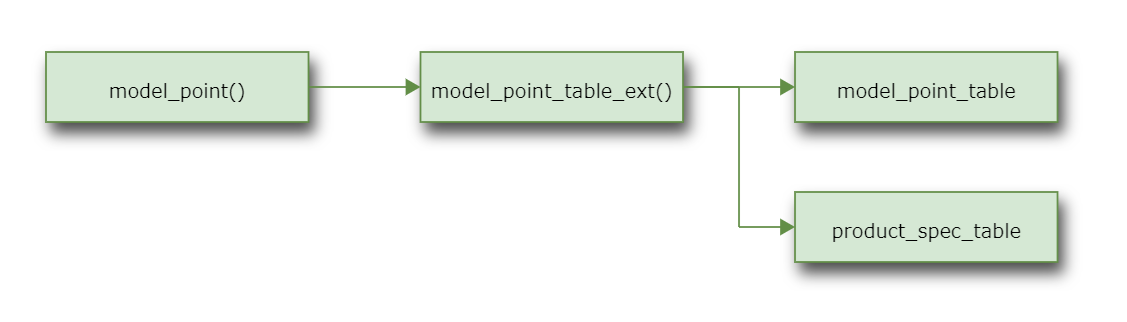
- product_spec_table#
Table of product specs
A DataFrame of product spec parameters by
spec_id.model_point_tableandproduct_spec_tablecolumns are joined inmodel_point_table_ext(), and theproduct_spec_tablecolumns become part of the model point attributes. Theproduct_spec_tablecolumns are read by the Cells with the same names as the columns:>>> Projection.product_spec_table premium_type has_surr_charge surr_charge_id load_prem_rate is_wl spec_id A SINGLE False NaN 0.10 False B SINGLE True type_1 0.00 False C LEVEL False NaN 0.10 True D LEVEL True type_3 0.05 True
Projection parameters#
This is a new business model and all model points are issued at time 0.
The time step of the model is monthly. Cashflows and other time-dependent
variables are indexed with t.
Cashflows and other flows that accumulate throughout a period
indexed with t denotes the sums of the flows from t til t+1.
Balance items indexed with t denotes the amount at t.
|
Projection length in months |
The max of all projection lengths |
Model point data#
The model point data is stored in an Excel file named model_point_table.xlsx under the model folder.
Target model points |
|
Extended model point table |
|
|
The sex of the model points |
The sum assured of the model points |
|
The policy term of the model points. |
|
|
The attained age at time t. |
The age at entry of the model points |
|
|
Duration of model points at |
|
Duration of model points at |
Whether surrender charge applies |
|
|
Whether the model point is whole life |
Rate of premium loading |
|
ID of surrender charge pattern |
|
Type of premium payment |
|
Initial account value per policy |
Assumptions#
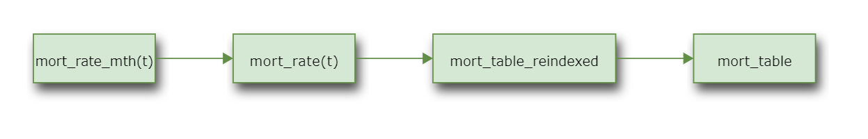
The mortality table is stored in an Excel file named mort_table.xlsx
under the model folder, and is read into mort_table as a DataFrame.
mort_table_reindexed() returns a mortality table
reshaped from mort_table, which is a Series
indexed with Age and Duration.
mort_rate() looks up mort_table_reindexed() and picks up
the annual mortality rates to be applied for all the
model points at time t and returns them in a Series.
mort_rate_mth() converts mort_rate() to the monthly mortality
rate to be applied during the month starting at time t.
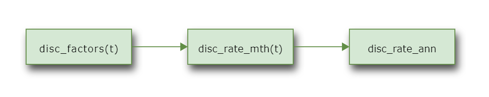
The discount rate data is stored in an Excel file named disc_rate_ann.xlsx
under the model folder, and is read into disc_rate_ann as a Series.
The lapse by duration is defined by a formula in lapse_rate().
expense_acq() holds the acquisition expense per policy at t=0.
expense_maint() holds the maintenance expense per policy per annum.
The maintenance expense inflates at a constant rate
of inflation given as inflation_rate().
The last age of mortality tables |
|
|
Mortality rate to be applied at time t |
Monthly mortality rate to be applied at time t |
|
MultiIndexed mortality table |
|
Discount factors. |
|
Monthly discount rate |
|
|
Lapse rate |
Acquisition expense per policy |
|
Annual maintenance expense per policy |
|
The inflation factor at time t |
|
Inflation rate |
Policy values#
By default, the amount of death benefit for each policy (claim_pp())
is set equal to sum_assured.
premium_pp() is the single premium amount if the model point
represents single premium policies (i.e. premium_type() is "SINGLE"),
or the monthly premium amount if the model point represents
level premium policies (i.e. premium_type() is "LEVEL").
|
Claim per policy |
|
Premium amount per policy |
Maintenance fee per account value |
|
|
Cost of insurance rate per account value |
Surrender charge rate |
|
Stacked surrender charge table |
|
maximum index of surrender charge table |
Policy decrement#
The policy decrement logic of CashValue_ME
is based on that of CashValue_SE.
except that each relevant formula operates on the entire model points.
|
Number of death |
|
Number of policies in-force |
|
Number of policies in-force |
Initial number of policies in-force |
|
|
Number of lapse |
Number of maturing policies |
|
|
Number of new business policies |
Account Value#
The account value logic of CashValue_ME
is based on CashValue_SE.
except that each relevant formula operates on the entire model points.
|
Investment income on account value |
Investment income on account value per policy |
|
Rate of investment return |
|
Table of investment return rates |
|
|
Account value per policy |
Net amount at risk per policy |
|
|
Cost of insurance charges per policy |
Per-policy premium portion put in the account value |
|
|
Maintenance fee per policy |
|
Account value in-force |
|
Premium portion put in account value |
|
Account value taken out to pay claim |
|
Claim in excess of account value |
|
Cost of insurance charges |
|
Maintenance fee deducted from account value |
|
Change in account value |
Check account value roll-forward |
Cashflows#
Cashflows are calculated as its per-policy amount times the number of policies.
The expense cashflow consists of acquisition expenses at issue and monthly maintenance expenses spent each month.
By default, commissions are defined as 5% premiums.
|
Surrender charge |
|
Claims |
|
Commissions |
|
Premium income |
|
Expenses |
|
Net cashflow |
Margin Analysis#
net_cf() can be expressed as the sum of expense and mortality
margins. The expense margin is defined as the sum of
premium loading, surrender charge and maintenance fees
net of commissions and expenses.
The mortality margin is defined coi() net of claims_over_av().
Expense margin |
|
Mortality margin |
|
Check consistency between net cashflow and margins |
Present values#
The Cells whose names start with pv_ are for calculating
the present values of the cashflows indicated by the rest of their names.
pv_pols_if() is not used
in CashValue_SE and BasicTerm_ME.
|
Present value of claims |
Present value of commissions |
|
Present value of expenses |
|
Present value of net cashflows. |
|
Present value of policies in-force |
|
Present value of premiums |
|
Present value of change in account value |
|
Present value of investment income |
|
Check present value summation |
Results#
result_cf() outputs the total cashflows of all the model points
as a DataFrame:
>>> result_cf()
          Premiums         Claims      Expenses   Commissions  Net Cashflow
0     1.002000e+08  795274.520511  2.016667e+06  5.010000e+06 -1.888257e+06
1     1.982432e+05  782659.768793  1.653397e+04  9.912161e+03  1.102781e+05
2     1.965019e+05  776554.840116  1.640233e+04  9.825093e+03  1.083123e+05
3     1.947758e+05  777512.879071  1.627174e+04  9.738790e+03  1.088861e+05
4     1.930649e+05  770406.958695  1.614219e+04  9.653245e+03  1.082080e+05
           ...            ...           ...           ...           ...
1136  0.000000e+00       0.000000  0.000000e+00  0.000000e+00  0.000000e+00
1137  0.000000e+00       0.000000  0.000000e+00  0.000000e+00  0.000000e+00
1138  0.000000e+00       0.000000  0.000000e+00  0.000000e+00  0.000000e+00
1139  0.000000e+00       0.000000  0.000000e+00  0.000000e+00  0.000000e+00
1140  0.000000e+00       0.000000  0.000000e+00  0.000000e+00  0.000000e+00

[1141 rows x 5 columns]
result_pv() outputs the present values of the cashflows by model points:
>>> result_pv()
              Premiums         Death  ...  Change in AV  Net Cashflow
poind_id                              ...
1         5.000000e+07  1.350327e+05  ...  3.771029e+06  4.957050e+06
2         5.000000e+07  1.608984e+06  ...  8.740610e+06  4.241619e+06
3         2.642236e+07  6.107771e+06  ...  1.104837e+07  6.058365e+06
4         2.201418e+07  1.329419e+07  ...  4.763115e+06  2.514042e+06

[4 rows x 9 columns]
Result table of cashflows |
|
Result table of present value of cashflows |
|
Result table of policy decrement |
Cells Descriptions#
- proj_len()[source]#
Projection length in months
proj_len()returns how many months the projection for each model point should be carried out for all the model point. Defined as:np.maximum(12 * policy_term() - duration_mth(0) + 1, 0)
Since this model carries out projections for all the model points simultaneously, the projections are actually carried out from 0 to
max_proj_lenfor all the model points.See also
- max_proj_len()#
The max of all projection lengths
Defined as
max(proj_len())See also
- model_point()[source]#
Target model points
Returns as a DataFrame the model points to be in the scope of calculation. By default, this Cells returns the entire
model_point_table_ext()without change.model_point_table_ext()is the extended model point table, which extendsmodel_point_tableby joining the columns inproduct_spec_table. Do not directly refer tomodel_point_tablein this formula. To select model points, change this formula so that this Cells returns a DataFrame that contains only the selected model points.Examples
To select only the model point 1:
def model_point():
    return model_point_table_ext().loc[1:1]
To select model points whose ages at entry are 40 or greater:
def model_point():
    return model_point_table[model_point_table_ext()["age_at_entry"] >= 40]
Note that the shape of the returned DataFrame must be the same as the original DataFrame, i.e.
model_point_table_ext().When selecting only one model point, make sure the returned object is a DataFrame, not a Series, as seen in the example above where
model_point_table_ext().loc[1:1]is specified instead ofmodel_point_table_ext().loc[1].Be careful not to accidentally change the original table held in
model_point_table_ext().See also
- model_point_table_ext()[source]#
Extended model point table
Returns an extended
model_point_tableby joiningproduct_spec_tableon thespec_idcolumn.See also
- sex()[source]#
The sex of the model points
Note
This cells is not used by default.
The
sexcolumn of the DataFrame returned bymodel_point().
- sum_assured()[source]#
The sum assured of the model points
The
sum_assuredcolumn of the DataFrame returned bymodel_point().
- policy_term()[source]#
The policy term of the model points.
The
policy_termcolumn of the DataFrame returned bymodel_point().
- age_at_entry()[source]#
The age at entry of the model points
The
age_at_entrycolumn of the DataFrame returned bymodel_point().
- duration_mth(t)[source]#
Duration of model points at
tin monthsIndicates how many months the policies have been in-force at
t. The initial values at time 0 are read from theduration_mthcolumn inmodel_point_tablethroughmodel_point(). Increments by 1 astincrements. Negative values ofduration_mth()indicate future new business policies. For example, If theduration_mth()is -15 at time 0, the model point is issued att=15.See also
- has_surr_charge()[source]#
Whether surrender charge applies
Trueif surrender charge on account value applies upon lapse,Falseif other wise. By default, the value is read from thehas_surr_chargecolumn inmodel_point().See also
- is_wl()[source]#
Whether the model point is whole life
Trueif the model point is whole life,Falseif other wise. By default, the value is read from theis_wlcolumn inmodel_point(). This attribute is used to determinpolicy_term(). IfTrue,policy_term()is defined asmort_table_last_age()minusage_at_entry(). IfFalse,policy_term()is read frommodel_point().See also
- load_prem_rate()[source]#
Rate of premium loading
This rate times
premium_pp()is collected from each premium and the rest is added to the account value.By default, the value is read from the
load_prem_ratecolumn inmodel_point().See also
- surr_charge_id()[source]#
ID of surrender charge pattern
A string to indicate the ID of the surrender charge pattern. The ID should be one of the column names in
surr_charge_tableifhas_surr_charge()isTrue.See also
Type of premium payment
Returns a string indicating the payment type, which is either
"LEVEL"if level payment, or"SINGLE"if single payment.
- av_pp_init()[source]#
Initial account value per policy
For existing business at time
0, returns initial per-policy accout value read from theav_pp_initcolumn inmodel_point(). For new business, 0 should be entered in the column.See also
- mort_table_last_age()[source]#
The last age of mortality tables
Returns the last age whose mortality rates are all 1. If no such age is found, return the last index of the tables
See also
- mort_rate(t)[source]#
Mortality rate to be applied at time t
Returns a Series of the mortality rates to be applied at time t. The index of the Series is
point_id, copied frommodel_point().
- mort_table_reindexed()[source]#
MultiIndexed mortality table
Returns a Series of mortlity rates reshaped from
mort_table. The returned Series is indexed by age and duration capped at 5.
- disc_factors()[source]#
Discount factors.
Vector of the discount factors as a Numpy array. Used for calculating the present values of cashflows.
See also
- disc_rate_mth()[source]#
Monthly discount rate
Nummpy array of monthly discount rates from time 0 to
max_proj_len()- 1 defined as:(1 + disc_rate_ann)**(1/12) - 1
See also
- lapse_rate(t)[source]#
Lapse rate
By default, the lapse rate assumption is defined by duration as:
max(0.1 - 0.02 * duration(t), 0.02)
See also
- inflation_rate()[source]#
Inflation rate
The inflation rate to be applied to the expense assumption. By defualt it is set to
0.01.See also
- claim_pp(t, kind)[source]#
Claim per policy
The claim amount per policy. The second parameter is to indicate the type of the claim, and it takes a string, which is either
"DEATH","LAPSE"or"MATURITY".The death benefit as denoted by
"DEATH", is the greater ofsum_assured()and mid-month account value (av_pp_at(t, "MID_MTH")).The surrender benefit as denoted by
"LAPSE"and the maturity benefit as denoted by"MATURITY"are equal to the mid-month account value.See also
Premium amount per policy
Single premium amount if
premium_type()is"SINGLE", monthly premium amount ifpremium_type()is"LEVEL".
- maint_fee_rate()[source]#
Maintenance fee per account value
The rate of maintenance fee on account value each month. Set to
0.01 / 12by default.See also
- coi_rate(t)[source]#
Cost of insurance rate per account value
The cost of insuranc rate per account value per month. By default, it is set to 1.1 times the monthly mortality rate.
See also
- surr_charge_rate(t)[source]#
Surrender charge rate
Surrender charge rate to be applied for lapsed policies
- surr_charge_table_stacked()[source]#
Stacked surrender charge table
surr_charge_tableconverted to a Series indexed with surrender charge ID and duration.See also
- surr_charge_max_idx()[source]#
maximum index of surrender charge table
The maximum index(duration) of
surr_charge_table.See also
- pols_if(t)[source]#
Number of policies in-force
pols_if(t)is an alias forpols_if_at(t, "BEF_MAT").See also
- pols_if_at(t, timing)[source]#
Number of policies in-force
pols_if_at(t, timing)calculates the number of policies in-force at timet. The second parametertimingtakes a string value to indicate the timing of in-force, which is either"BEF_MAT","BEF_NB"or"BEF_DECR".BEF_MAT
The number of policies in-force before maturity after lapse and death. At time 0, the value is read from
pols_if_init(). For time > 0, defined as:pols_if_at(t-1, "BEF_DECR") - pols_lapse(t-1) - pols_death(t-1)
BEF_NB
The number of policies in-force before new business after maturity. Defined as:
pols_if_at(t, "BEF_MAT") - pols_maturity(t)
BEF_DECR
The number of policies in-force before lapse and death after new business. Defined as:
pols_if_at(t, "BEF_NB") + pols_new_biz(t)
- pols_if_init()[source]#
Initial number of policies in-force
Number of in-force policies at time 0 referenced from
pols_if_at(0, "BEF_MAT").
- pols_lapse(t)[source]#
Number of lapse
Number of policies decreased by lapse during
tandt+1.See also
- pols_maturity(t)[source]#
Number of maturing policies
The policy maturity occurs when
duration_mth()equals 12 timespolicy_term(). The amount is equal topols_if_at(t, "BEF_MAT").otherwise
0.
- pols_new_biz(t)[source]#
Number of new business policies
The number of new business policies. The value
duration_mth(0)for the selected model point is read from thepolicy_countcolumn inmodel_point(). If the value is 0 or negative, the model point is new business at t=0 or at t whenduration_mth(t)is 0, and thepols_new_biz(t)is read from thepolicy_countinmodel_point().See also
- inv_income(t)[source]#
Investment income on account value
Investment income earned on account value during each period. For the plicies decreased by lapse and death, half the investment income is credited.
- inv_income_pp(t)[source]#
Investment income on account value per policy
Investment income on account value defined as:
inv_return_mth(t) * av_pp_at(t, "BEF_INV")
See also
- inv_return_mth(t)[source]#
Rate of investment return
Rate of monthly investment return for
scen_idandtread frominv_return_table()See also
- inv_return_table()[source]#
Table of investment return rates
Returns a Series of monthly investment retuns. The Series is indexed with
scen_idandtwhich is inherited fromstd_norm_rand.\[\exp\left(\left(\mu-\frac{\sigma^{2}}{2}\right)\Delta{t}+\sigma\sqrt{\Delta{t}}\epsilon\right)-1\]where \(\mu=2\%\), \(\sigma=3\%\), \(\Delta{t}=\frac{1}{12}\), and \(\epsilon\) is a randome number from the standard normal distribution.
See also
- av_pp_at(t, timing)[source]#
Account value per policy
av_at(t, timing)calculates the total amount of account value at timetfor the policies in-force.At each
t, the events that change the account value balance occur in the following order:Premium payment
Fee deduction
Investment income is assumed to be earned throughout each month, so at the middle of the month when death and lapse occur, half the investment income for the month is credited.
The second parameter
timingtakes a string to indicate the timing of the account value, which is either"BEF_PREM","BEF_FEE","BEF_INV"or"MID_MTH".BEF_PREM
Account value before premium payment. At the start of the projection (i.e. when
t=0), the account value is set toav_pp_init().BEF_FEE
Account value after premium payment before fee deduction
BEF_INV
Account value after fee deduction before crediting investemnt return
MID_MTH
Account value at middle of month (
t+0.5) when half the investment retun for the month is credited
- net_amt_at_risk(t)[source]#
Net amount at risk per policy
Return sum assured net of account value per policy.
See also
- coi_pp(t)[source]#
Cost of insurance charges per policy
The cost of insurance charges per policy. Defined as the coi charge rate times net amount at risk per policy.
See also
- prem_to_av_pp(t)[source]#
Per-policy premium portion put in the account value
The amount of premium per policy net of loading, which is put in the accoutn value.
See also
- av_at(t, timing)[source]#
Account value in-force
av_at(t, timing)calculates the total amount of account value at timetfor the policies represented by a model point.At each
t, the events that change the account value balance occur in the following order:Maturity
New business and premium payment
Fee deduction
The second parameter
timingtakes a string to indicate the timing of the account value, which is either"BEF_MAT","BEF_NB"or"BEF_FEE".BEF_MAT
The amount of account value before maturity, defined as:
av_pp_at(t, "BEF_PREM") * pols_if_at(t, "BEF_MAT")
BEF_NB
The amount of account value before new business after maturity, defined as:
av_pp_at(t, "BEF_PREM") * pols_if_at(t, "BEF_NB")
BEF_FEE
The amount of account value before lapse and death after new business, defined as:
av_pp_at(t, "BEF_FEE") * pols_if_at(t, "BEF_DECR")
See also
- prem_to_av(t)[source]#
Premium portion put in account value
The amount of premiums net of loadings, which is put in the accoutn value.
See also
- claims_from_av(t, kind)[source]#
Account value taken out to pay claim
The part of the claim amount that is paid from account value. The second parameter takes a string indicating the type of the claim, which is either
"DEATH","LAPSE"or"MATURITY".Death benefit is denoted by
"DEATH", is defined as:av_pp_at(t, "MID_MTH") * pols_death(t)
When the account value is greater than the death benefit, the death benefit equates to the account value.
Surrender benefit as denoted by
"LAPSE"is defined as:av_pp_at(t, "MID_MTH") * pols_lapse(t)
As the surrender benefit is defined as account value less surrender charge, when there is no surrender charge the surrender benefit equates to the account value.
Maturity benefit as denoted by
"MATURITY"is defined as:av_pp_at(t, "BEF_PREM") * pols_maturity(t)
By default, the maturity benefit equates to the account value of maturing policies.
- claims_over_av(t, kind)[source]#
Claim in excess of account value
The amount of death benefits in excess of account value.
coi()net of this amount represents mortality margin.See also
- coi(t)[source]#
Cost of insurance charges
The cost of insurance charges deducted from acccount values each period.
See also
- av_change(t)[source]#
Change in account value
Change in account value during each period, defined as:
av_at(t+1, 'BEF_MAT') - av_at(t, 'BEF_MAT')
See also
- check_av_roll_fwd()[source]#
Check account value roll-forward
Returns
Tureifav_at(t+1, "BEF_NB")equates to the following expression for allt, otherwise returnsFalse:av_at(t, "BEF_MAT") + prem_to_av(t) - maint_fee(t) - coi(t) + inv_income(t) - claims_from_av(t, "DEATH") - claims_from_av(t, "LAPSE") - claims_from_av(t, "MATURITY"))
- surr_charge(t)[source]#
Surrender charge
Surrender charge rate times account values of lapsed policies
- claims(t, kind=None)[source]#
Claims
The claim amount during the period from
ttot+1. The optional second parameter is for indicating the type of the claim, and it takes a string, which is either"DEATH","LAPSE"or"MATURITY", or defaults toNoneto indicate the total of all the types of claims during the period.The death benefit as denoted by
"DEATH"is defined as:claim_pp(t) * pols_death(t)
The surrender benefit as denoted by
"LAPSE"is defined as:claims_from_av(t, "LAPSE") - surr_charge(t)
The maturity benefit as denoted by
"MATURITY"is defined as:claims_from_av(t, "MATURITY")
- commissions(t)[source]#
Commissions
By default, 100% premiums for the first year, 0 otherwise.
See also
Premium income
Premium income during the period from
ttot+1defined as:premium_pp() * pols_if_at(t, "BEF_DECR")
See also
- expenses(t)[source]#
Expenses
Expenses during the period from
ttot+1defined as the sum of acquisition expenses and maintenance expenses. The acquisition expenses are modeled asexpense_acq()timespols_new_biz(). The maintenance expenses are modeled asexpense_maint()timesinflation_factor()timespols_if_at()before decrement.
- net_cf(t)[source]#
Net cashflow
Net cashflow for the period from
ttot+1defined as:premiums(t) - claims(t) - expenses(t) - commissions(t)
See also
- margin_expense(t)[source]#
Expense margin
Expense margin is defined as the sum of premium loading, surrender charge and maintenance fees net of commissions and expenses.
The sum of the expense margin and mortality margin add up to the net cashflow.
- margin_mortality(t)[source]#
Mortality margin
Mortality margin is defined
coi()net ofclaims_over_av().The sum of the expense margin and mortality margin add up to the net cashflow.
See also
- check_margin()[source]#
Check consistency between net cashflow and margins
Returns
Trueifnet_cf()equates to the sum ofmargin_expense()andmargin_mortality()for allt, otherwise, returnsFalse.See also
- pv_net_cf()[source]#
Present value of net cashflows.
Defined as:
pv_premiums() + pv_inv_income()
- pv_claims() - pv_expenses() - pv_commissions() - pv_av_change()
- pv_pols_if()[source]#
Present value of policies in-force
Note
This cells is not used by default.
The discounted sum of the number of in-force policies at each month. It is used as the annuity factor for calculating
net_premium_pp().
Present value of premiums
See also
- pv_inv_income()[source]#
Present value of investment income
The discounted sum of monthly investment income.
See also
- check_pv_net_cf()[source]#
Check present value summation
Check if the present value of
net_cf()matches the sum of the present values of each cashflow. Returns the check result asTrueorFalse.See also