Selecting model points by cluster analysis#
This notebook applies cluster analysis to model point selection. More specifically, we use the k-means method to partition a sample portfolio of seriatim policies and select representative model points.
As the sample portfolio, we use 10,000 seriatim term policies and their projection results, such as cashflows and present values of the cashflows. The sample policies are generated by a jupyter notebook included in the cluster library. The model used for generating the cashflows and present values are derived from BasicTerm_ME in the basiclife library, and included in the cluster library.
What is the target use case?
What should we look at to validate results?
What should we use for variables ?
What should the number of representative model points be?
What initializataion method should we use for k-means?
Target use case
The target use case for this exercise is when we want to run deterministic projections of a large block of protection business under many different sensitivity scenarios.
We construct a proxy portfolio based on the seriatim projection result of a base scenario by selecting and scaling representative polices. If the policy attributes of the proxy portfolio and projections results under the sensitivity scenarios obtained by using the proxy are close enough to those of the seriatim policies, then we can use the proxy portfolio for running the sensitivities and save time and computing resources.
In this exercise, we do not cover the cases where stochastic runs are involved. In reliaity, the stochastic cases would benefit more from the reduction in time and computing resources.
Target metrics
To determine how closely selected policies represents the seriatim policies, we look at the following figures:
Net cashflows
Policy attributes, such as issue age, policy term, sum assured and duration.
Presnet value of net cashflows and their components.
Among the above, the most important metric would be the present value of net cashflows, as it often represents the whole or a major part of insurance liabilities. In practice, the maximum allowable error in the estimation of the present value of cashflows should be specified (e.g. 1%).
Choice of variables
The k-means method partitions samples based on squared Euclidean distances between samples. Samples are vectors of variable values. What we choose for the variables has significant impact on the results. The chosen variables are more accurately estimated by the proxy portfolio. In this exercise, we test the following 3 types of variables and compare the results.
Net cashflows
Policy attributes
Present values of net cashflows and their components
Although not covered in this exercise, combinations of variables chosen across the 3 types above may yield better results. Further tests are left to subsequent studies.
Reduction ratio
Reduction ratio is defined as the number of seriatim policies devided by the number of selected representative model points. The higher the ratio is, the more effective the proxy portfolio is. In this exercise, we select 1000 model points out of 10,000, so the ratio in 10. The ratio and the accuracy of the proxy is a trade-off. Furthur tests beyond this exercise are desired to see how high the ratio we can get while maintaiing a certain level of accuracy.
Initialization method
The k-means method returns diffrent outcomes depending on their initial values of cluster centroids. How to select the initial values is an area to be furthur explored, but in this exercise, we simply use the default method provided by sciki-learn.
References:
Gan, G. and Valdez, E. A. (2019). Data Clustering with Actuarial Applications
Goto, Y. A method to determine model points with cluster analysis, Virtual ICA 2018
Milliman. Cluster analysis: A spatial approach to actuarial modeling
Click the badge below to run this notebook online on Google Colab. You need a Google account and need to be logged in to it to run this notebook on Google Colab. ![]()
The next code cell below is relevant only when you run this notebook on Google Colab. It installs lifelib and creates a copy of the library for this notebook.
[1]:
import sys, os

if 'google.colab' in sys.modules:
    lib = 'cluster'; lib_dir = '/content/'+ lib
    if not os.path.exists(lib_dir):
        !pip install lifelib
        import lifelib; lifelib.create(lib, lib_dir)

    %cd $lib_dir
The next code imports the necessary Python modules.
[2]:
import numpy as np
import pandas as pd
from sklearn.cluster import KMeans
from sklearn.metrics import pairwise_distances_argmin_min, r2_score
import matplotlib.cm
import matplotlib.pyplot as plt
Sample Data#
3 types of data are used, which are policy data, cashflow data and present value data. The policy data is in one file, while each of the other two consists of 3 sets of files, which correspond to the base, lapse-stress, and mortality-stress scenarios.
The base cashflows and present values are used for calibration, while the cashflows and present values of the stressed scenarios are not.
Cashflow Data#
3 sets of cashflow data are read from Excel files into DataFrames. The DataFrames are assigned to these 3 global variables:
cfs: The base scenariocsf_lapse50: The stress scenario of 50% level increase in lapse ratescfs_mort15: The stress scenario of 15% level increase in mortality rates
In each file, net annual cashflows of the 10,000 sample policies are included. The files are outputs of net_cf_annual in BasicTerm_ME_for_Cluster.
[3]:
cfs = pd.read_excel('cashflows_seriatim_10K.xlsx', index_col=0)
cfs_lapse50 = pd.read_excel('cashflows_seriatim_10K_lapse50.xlsx', index_col=0)
cfs_mort15 = pd.read_excel('cashflows_seriatim_10K_mort15.xlsx', index_col=0)
cfs_list = [cfs, cfs_lapse50, cfs_mort15]
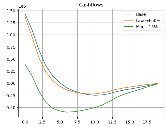
The chart below compares the shapes of the 3 aggregated cashflows.
[4]:
pd.DataFrame.from_dict({
    'Base': cfs.sum(),
    'Lapse+50%': cfs_lapse50.sum(),
    'Mort+15%': cfs_mort15.sum()}).plot(grid=True, title='Cashflows')
[4]:
<Axes: title={'center': 'Cashflows'}>
Policy Data#
Policy data is read from an Excel file into a DataFrame. In this sample case, 4 attributes completely defines a policy, so only the attributes are extracted as columns of the DataFrame. The DataFrame is then assigned to pol_data.
[5]:
pol_data = pd.read_excel(
    'BasicTerm_ME_for_Cluster/model_point_table.xlsx', index_col=0
)[['age_at_entry', 'policy_term', 'sum_assured', 'duration_mth']]
pol_data
[5]:
| age_at_entry | policy_term | sum_assured | duration_mth | |
|---|---|---|---|---|
| policy_id | ||||
| 1 | 47 | 10 | 622000 | 28 |
| 2 | 29 | 20 | 752000 | 213 |
| 3 | 51 | 10 | 799000 | 39 |
| 4 | 32 | 20 | 422000 | 140 |
| 5 | 28 | 15 | 605000 | 76 |
| ... | ... | ... | ... | ... |
| 9996 | 47 | 20 | 827000 | 168 |
| 9997 | 30 | 15 | 826000 | 169 |
| 9998 | 45 | 20 | 783000 | 158 |
| 9999 | 39 | 20 | 302000 | 41 |
| 10000 | 22 | 15 | 576000 | 167 |
10000 rows × 4 columns
Present Value Data#
For each of the 3 scnarios, the present values of the net cashflowand their components are read from an Excel file into a DataFrame. The components are the present values of premiums, claims, expenses and commissions. The DataFrames are assigned to these 3 global variables:
pvs: The base scenariopvs_lapse50: The stress scenario of 50% level increase in lapse ratespvs_mort15: The stress scenario of 15% level increase in mortality rates
In each file, net annual cashflows of the 10,000 sample policies are included. The files are outputs of result_pv in BasicTerm_ME_for_Cluster. The discount rate used is flat 3%.
[6]:
pvs = pd.read_excel('pv_seriatim_10K.xlsx', index_col=0)
pvs_lapse50 = pd.read_excel('pv_seriatim_10K_lapse50.xlsx', index_col=0)
pvs_mort15 = pd.read_excel('pv_seriatim_10K_mort15.xlsx', index_col=0)
pvs_list = [pvs, pvs_lapse50, pvs_mort15]
pvs
[6]:
| pv_premiums | pv_claims | pv_expenses | pv_commissions | pv_net_cf | |
|---|---|---|---|---|---|
| policy_id | |||||
| 1 | 5117.931213 | 3786.367310 | 278.536674 | 0.0 | 1053.027229 |
| 2 | 1563.198303 | 1733.892221 | 129.198252 | 0.0 | -299.892170 |
| 3 | 8333.617576 | 6646.840127 | 270.360068 | 0.0 | 1416.417381 |
| 4 | 3229.275711 | 3098.020912 | 424.560625 | 0.0 | -293.305825 |
| 5 | 3203.527395 | 2653.011845 | 401.855897 | 0.0 | 148.659654 |
| ... | ... | ... | ... | ... | ... |
| 9996 | 11839.037487 | 13872.879725 | 318.025035 | 0.0 | -2351.867273 |
| 9997 | 662.104216 | 670.314857 | 54.077923 | 0.0 | -62.288565 |
| 9998 | 10887.623809 | 12130.102842 | 356.697457 | 0.0 | -1599.176490 |
| 9999 | 4041.577020 | 2997.112776 | 522.558913 | 0.0 | 521.905331 |
| 10000 | 403.672732 | 379.494165 | 63.704186 | 0.0 | -39.525618 |
10000 rows × 5 columns
Python Code#
Clusters, a class to facilitate the calibration process is defined below. The Clusters class wraps the fitted KMeans object which is calibrated using variables given as loc_vars through its initializer.
We use the KMeans class imported from scikit-learn library in the initializer of the Clusters class. The fit method on a KMeans object returns the object fitted using the local variables given to the method.
We use the pairwise_distances_argmin_min method from sckit-learn to find the samples closest to the centroids of the fitted KMeans object.
The labels_ property of the fitted KMeans object holds cluster ID for each sample, indicating which cluster each sample belongs to.
[7]:
class Clusters:

    def __init__(self, loc_vars):

        self.kmeans = kmeans = KMeans(n_clusters=1000, random_state=0, n_init=10).fit(np.ascontiguousarray(loc_vars))
        closest, _ = pairwise_distances_argmin_min(kmeans.cluster_centers_, np.ascontiguousarray(loc_vars))

        rep_ids = pd.Series(data=(closest+1))   # 0-based to 1-based indexes
        rep_ids.name = 'policy_id'
        rep_ids.index.name = 'cluster_id'
        self.rep_ids = rep_ids

        self.policy_count = self.agg_by_cluster(pd.DataFrame({'policy_count': [1] * len(loc_vars)}))['policy_count']

    def agg_by_cluster(self, df, agg=None):
        """Aggregate columns by cluster"""
        temp = df.copy()
        temp['cluster_id'] = self.kmeans.labels_
        temp = temp.set_index('cluster_id')
        agg = {c: (agg[c] if c in agg else 'sum') for c in temp.columns} if agg else "sum"
        return temp.groupby(temp.index).agg(agg)

    def extract_reps(self, df):
        """Extract the rows of representative policies"""
        temp = pd.merge(self.rep_ids, df.reset_index(), how='left', on='policy_id')
        temp.index.name = 'cluster_id'
        return temp.drop('policy_id', axis=1)

    def extract_and_scale_reps(self, df, agg=None):
        """Extract and scale the rows of representative policies"""
        if agg:
            cols = df.columns
            mult = pd.DataFrame({c: (self.policy_count if (c not in agg or agg[c] == 'sum') else 1) for c in cols})
            return self.extract_reps(df).mul(mult)
        else:
            return self.extract_reps(df).mul(self.policy_count, axis=0)

    def compare(self, df, agg=None):
        """Returns a multi-indexed Dataframe comparing actual and estimate"""
        source = self.agg_by_cluster(df, agg)
        target = self.extract_and_scale_reps(df, agg)
        return pd.DataFrame({'actual': source.stack(), 'estimate':target.stack()})

    def compare_total(self, df, agg=None):
        """Aggregate ``df`` by columns"""
        if agg:
            cols = df.columns
            op = {c: (agg[c] if c in agg else 'sum') for c in df.columns}
            actual = df.agg(op)
            estimate = self.extract_and_scale_reps(df, agg=op)

            op = {k: ((lambda s: s.dot(self.policy_count) / self.policy_count.sum()) if v == 'mean' else v) for k, v in op.items()}
            estimate = estimate.agg(op)

        else:
            actual = df.sum()
            estimate = self.extract_and_scale_reps(df).sum()

        return pd.DataFrame({'actual': actual, 'estimate': estimate, 'error': estimate / actual - 1})
The functions below are for outputting plots.
[8]:
def generate_subplots(count, shape):
    "Generator to output multiple charts in subplots"

    row_count, col_count = shape
    size_x, size_y = plt.rcParams['figure.figsize']
    size_x, size_y = size_x * col_count, size_y * row_count

    fig, axs = plt.subplots(row_count, col_count, figsize=(size_x, size_y))
    fig.tight_layout(pad=3)

    for i in range(count):
        r = i // col_count
        c = i - r * col_count
        ax = axs[r, c] if (row_count > 1 and col_count > 1) else axs[r] if row_count > 1 else axs[c] if col_count > 1 else axs
        ax.grid(True)
        yield ax


def plot_colored_scatter(ax, df, title=None):
    """Draw a scatter plot in different colours by level-1 index

    ``df`` should be a DataFrame returned by the compare method.
    """

    colors = matplotlib.cm.rainbow(np.linspace(0, 1, len(df.index.levels[1])))

    for y, c in zip(df.index.levels[1], colors):
        ax.scatter(df.xs(y, level=1)['actual'], df.xs(y, level=1)['estimate'], color=c, s=9)

    ax.set_xlabel('actual')
    ax.set_ylabel('estimate')
    if title:
        ax.set_title(title)
    ax.grid(True)
    draw_identity_line(ax)


def plot_separate_scatter(df, row_count, col_count):
    """Draw multiple scatter plot with R-squared

    ``df`` should be a DataFrame returned by the compare method.
    """
    names = df.index.levels[1]
    count = len(names)

    size_x, size_y = plt.rcParams['figure.figsize']
    size_x, size_y = size_x * col_count, size_y * row_count

    for i, ax in enumerate(generate_subplots(count, (row_count, col_count))):
        df_n = df.xs(names[i], level=1)
        df_n.plot(x='actual', y='estimate', kind='scatter', ax=ax, title=names[i], grid=True)
        draw_identity_line(ax)

        # Add R2 in upper left corner
        r2_x = 0.95 * ax.get_xlim()[0] + 0.05 * ax.get_xlim()[1]
        r2_y = 0.05 * ax.get_ylim()[0] + 0.95 * ax.get_ylim()[1]
        ax.text(r2_x, r2_y, 'R2: {:.1f}%'.format(calc_r2_score(df_n) * 100), verticalalignment='top')


def draw_identity_line(ax):
    lims = [
        np.min([ax.get_xlim(), ax.get_ylim()]),  # min of both axes
        np.max([ax.get_xlim(), ax.get_ylim()]),  # max of both axes
    ]
    # now plot both limits against eachother
    ax.plot(lims, lims, 'r-', linewidth=0.5)
    ax.set_xlim(lims)
    ax.set_ylim(lims)


def calc_r2_score(df):
    "Return R-squared between actual and estimate columns"
    return r2_score(df['actual'], df['estimate'])
Cashflow Calibration#
The first calibration approach we test is to use base annual cashflows as calibration variables.
[9]:
cluster_cfs = Clusters(cfs)
Cashflow Analysis#
Below the total net cashflows under the base scenario are compared between actual, which denotes the total net cashflows of the seriatim sample policies, and estimate, which denots the total net cashflows calculated as the net cashflows of the selected representative policies multiplied by the numbers of policies in the clusters.
[10]:
cluster_cfs.compare_total(cfs)
[10]:
| actual | estimate | error | |
|---|---|---|---|
| 0 | 1.435932e+06 | 1.436594e+06 | 0.000461 |
| 1 | 1.105742e+06 | 1.110914e+06 | 0.004677 |
| 2 | 6.820530e+05 | 6.788524e+05 | -0.004693 |
| 3 | 3.579056e+05 | 3.572310e+05 | -0.001885 |
| 4 | 1.450520e+05 | 1.499286e+05 | 0.033620 |
| 5 | 3.343158e+03 | 1.358889e+04 | 3.064687 |
| 6 | -9.917748e+04 | -9.420853e+04 | -0.050102 |
| 7 | -1.636027e+05 | -1.593145e+05 | -0.026211 |
| 8 | -2.099648e+05 | -2.013429e+05 | -0.041063 |
| 9 | -2.391351e+05 | -2.358902e+05 | -0.013570 |
| 10 | -2.521441e+05 | -2.505832e+05 | -0.006191 |
| 11 | -2.458585e+05 | -2.438153e+05 | -0.008310 |
| 12 | -2.214476e+05 | -2.176521e+05 | -0.017140 |
| 13 | -1.802033e+05 | -1.772599e+05 | -0.016334 |
| 14 | -1.492649e+05 | -1.459876e+05 | -0.021956 |
| 15 | -1.242241e+05 | -1.224347e+05 | -0.014404 |
| 16 | -9.948838e+04 | -9.926656e+04 | -0.002230 |
| 17 | -7.169144e+04 | -7.182005e+04 | 0.001794 |
| 18 | -4.188922e+04 | -3.896544e+04 | -0.069798 |
| 19 | -1.398866e+04 | -1.276479e+04 | -0.087490 |
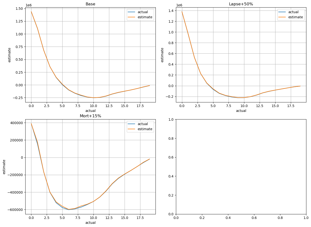
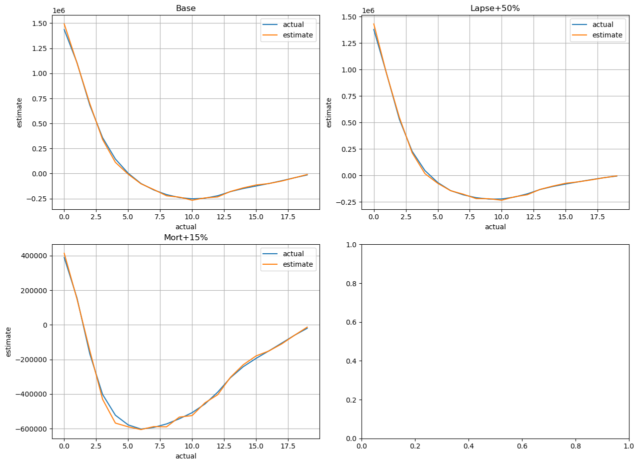
The charts below visualize how well the estimated cashflows match the actual.
[11]:
def plot_cashflows(ax, cfs, title=None):
    "Draw line plots of cashflows"
    cfs[['actual', 'estimate']].plot(ax= ax, grid=True, title=title, xlabel='actual', ylabel='estimate')

scen_titles = ['Base', 'Lapse+50%', 'Mort+15%']
for ax, df, title in zip(generate_subplots(3, (2, 2)), cfs_list, scen_titles):
    plot_cashflows(ax, cluster_cfs.compare_total(df), title)
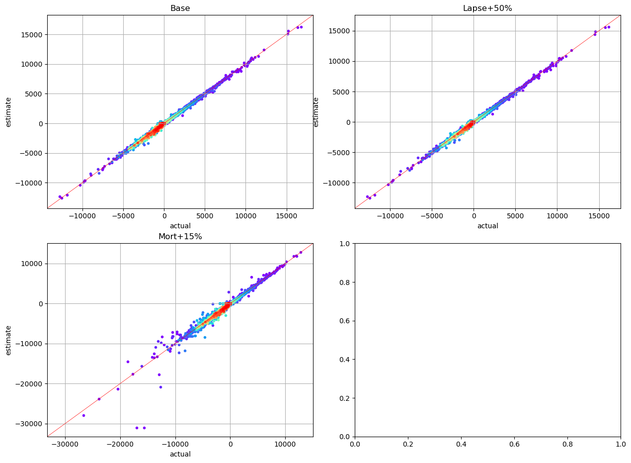
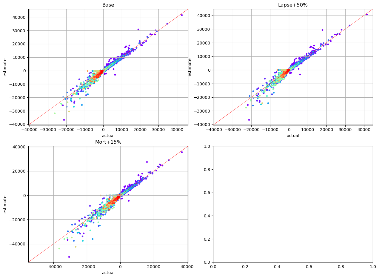
The scatter charts below plots net annual cashflows by cluster. The read plots represent the nearest cashflows while violet plots are the farthest.
[12]:
for ax, df, title in zip(generate_subplots(3, (2, 2)), cfs_list, scen_titles):
    plot_colored_scatter(ax, cluster_cfs.compare(df), title=title)
Policy Attribute Analysis#
[13]:
mean_attrs = {'age_at_entry':'mean', 'policy_term':'mean', 'duration_mth':'mean'}
cluster_cfs.compare_total(pol_data, agg=mean_attrs)
[13]:
| actual | estimate | error | |
|---|---|---|---|
| age_at_entry | 3.937720e+01 | 3.805530e+01 | -0.033570 |
| policy_term | 1.493600e+01 | 1.499350e+01 | 0.003850 |
| sum_assured | 5.060517e+09 | 5.313966e+09 | 0.050084 |
| duration_mth | 8.977470e+01 | 9.064560e+01 | 0.009701 |
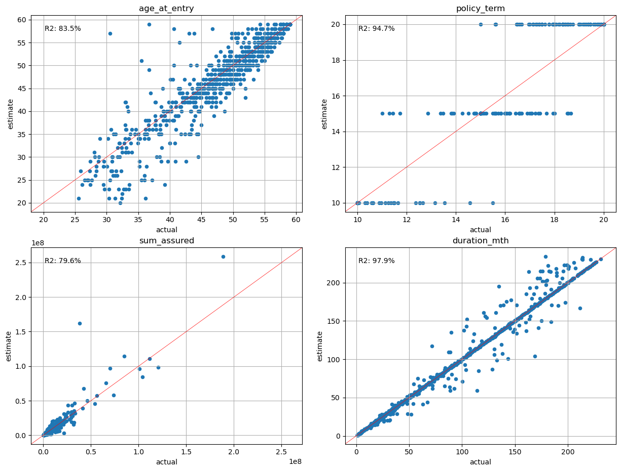
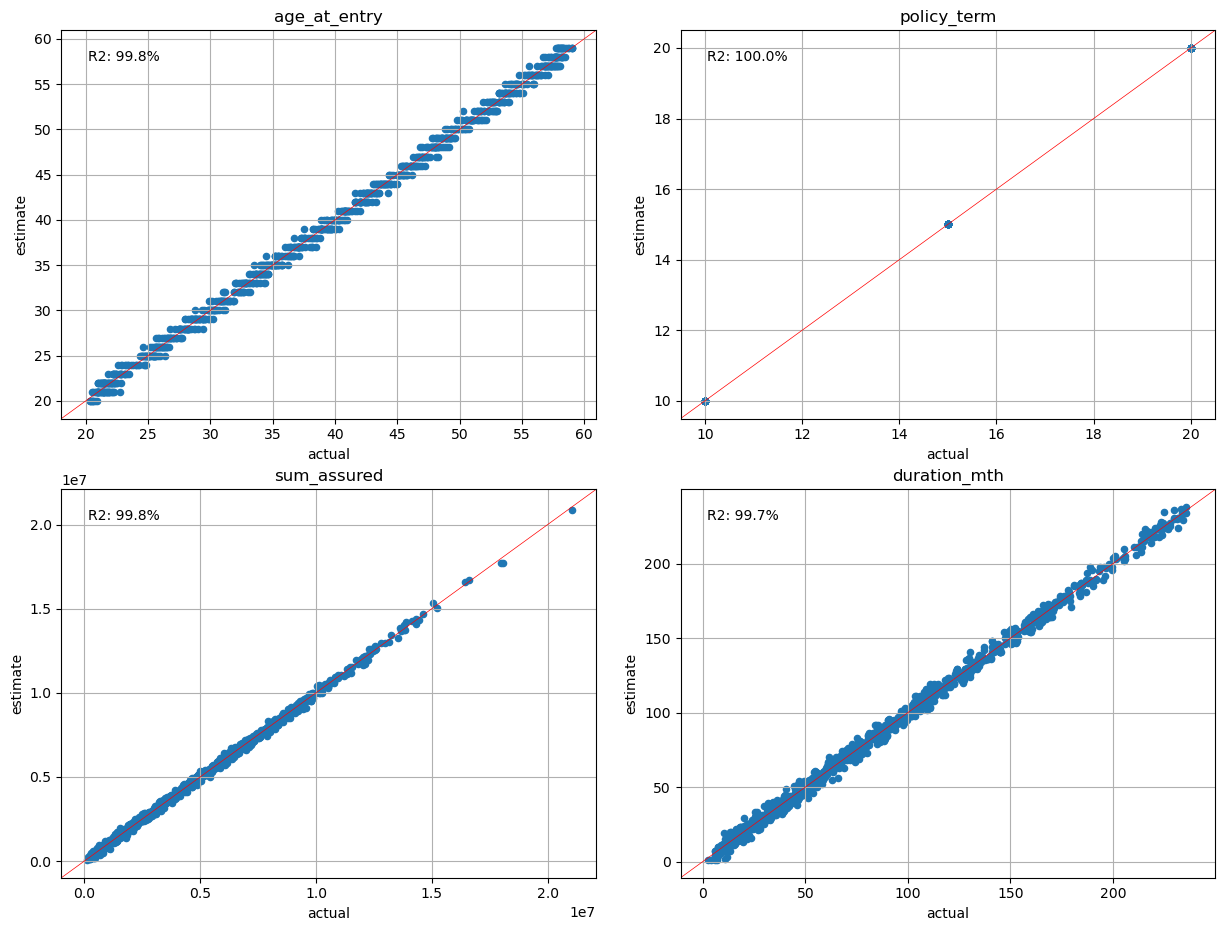
The charts below visualize how well the estimated policy attributes match the actual by cluster. The age_at_entry, policy_term and duration_mth charts plot the average of them in each cluster, while the sum_assured chart plots the total of each cluster. The X axises represent the acutual values, while the Y axises represent the estimated values.
[14]:
plot_separate_scatter(cluster_cfs.compare(pol_data, agg=mean_attrs), 2, 2)
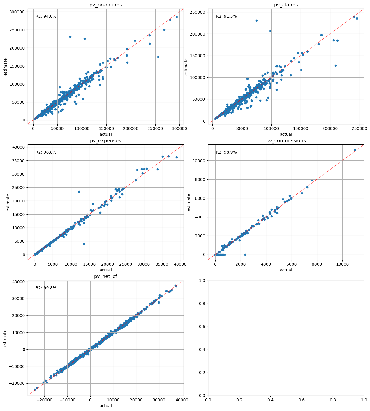
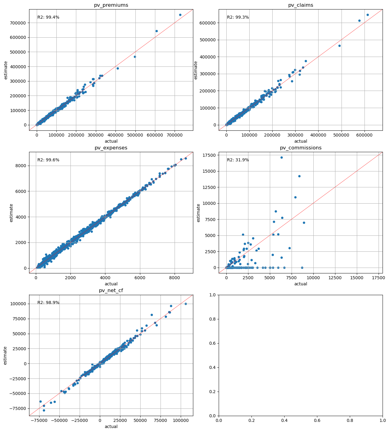
Present Value Analysis#
The present values of the net cashflows and their components are estimated and compared against the seriatim results for each scenario.
[15]:
cluster_cfs.compare_total(pvs)
[15]:
| actual | estimate | error | |
|---|---|---|---|
| pv_premiums | 4.860639e+07 | 4.841394e+07 | -0.003959 |
| pv_claims | 4.331937e+07 | 4.308694e+07 | -0.005365 |
| pv_expenses | 2.949823e+06 | 2.951866e+06 | 0.000693 |
| pv_commissions | 2.748443e+05 | 2.679155e+05 | -0.025210 |
| pv_net_cf | 2.062353e+06 | 2.107214e+06 | 0.021752 |
[16]:
cluster_cfs.compare_total(pvs_lapse50)
[16]:
| actual | estimate | error | |
|---|---|---|---|
| pv_premiums | 4.280459e+07 | 4.258599e+07 | -0.005107 |
| pv_claims | 3.831786e+07 | 3.806856e+07 | -0.006506 |
| pv_expenses | 2.579405e+06 | 2.579459e+06 | 0.000021 |
| pv_commissions | 2.653036e+05 | 2.585908e+05 | -0.025302 |
| pv_net_cf | 1.642024e+06 | 1.679376e+06 | 0.022747 |
[17]:
cluster_cfs.compare_total(pvs_mort15)
[17]:
| actual | estimate | error | |
|---|---|---|---|
| pv_premiums | 4.853083e+07 | 4.834040e+07 | -0.003924 |
| pv_claims | 4.973258e+07 | 4.946751e+07 | -0.005330 |
| pv_expenses | 2.946908e+06 | 2.949144e+06 | 0.000759 |
| pv_commissions | 2.748356e+05 | 2.679072e+05 | -0.025209 |
| pv_net_cf | -4.423494e+06 | -4.344168e+06 | -0.017933 |
[18]:
plot_separate_scatter(cluster_cfs.compare(pvs), 3, 2)
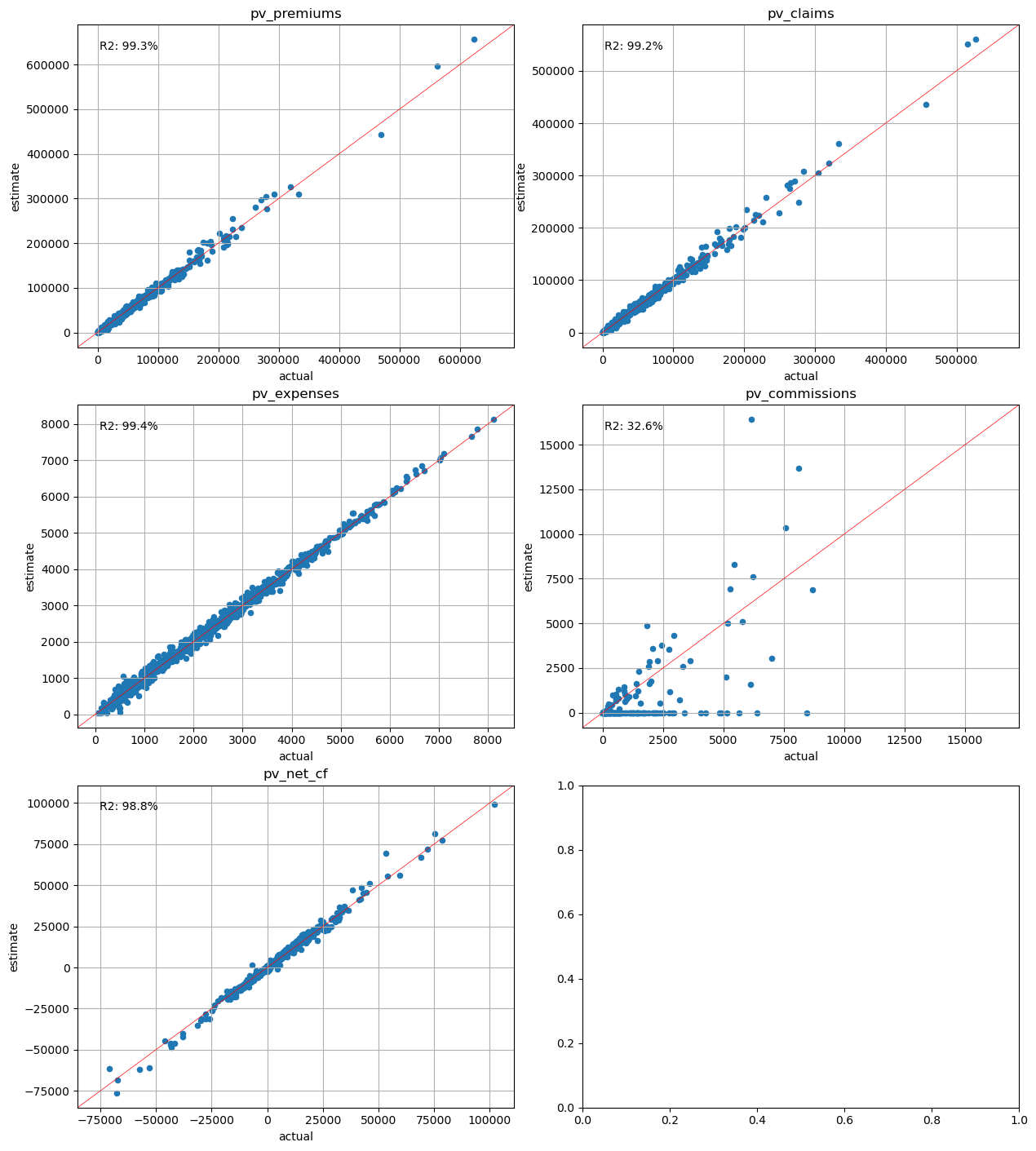
[19]:
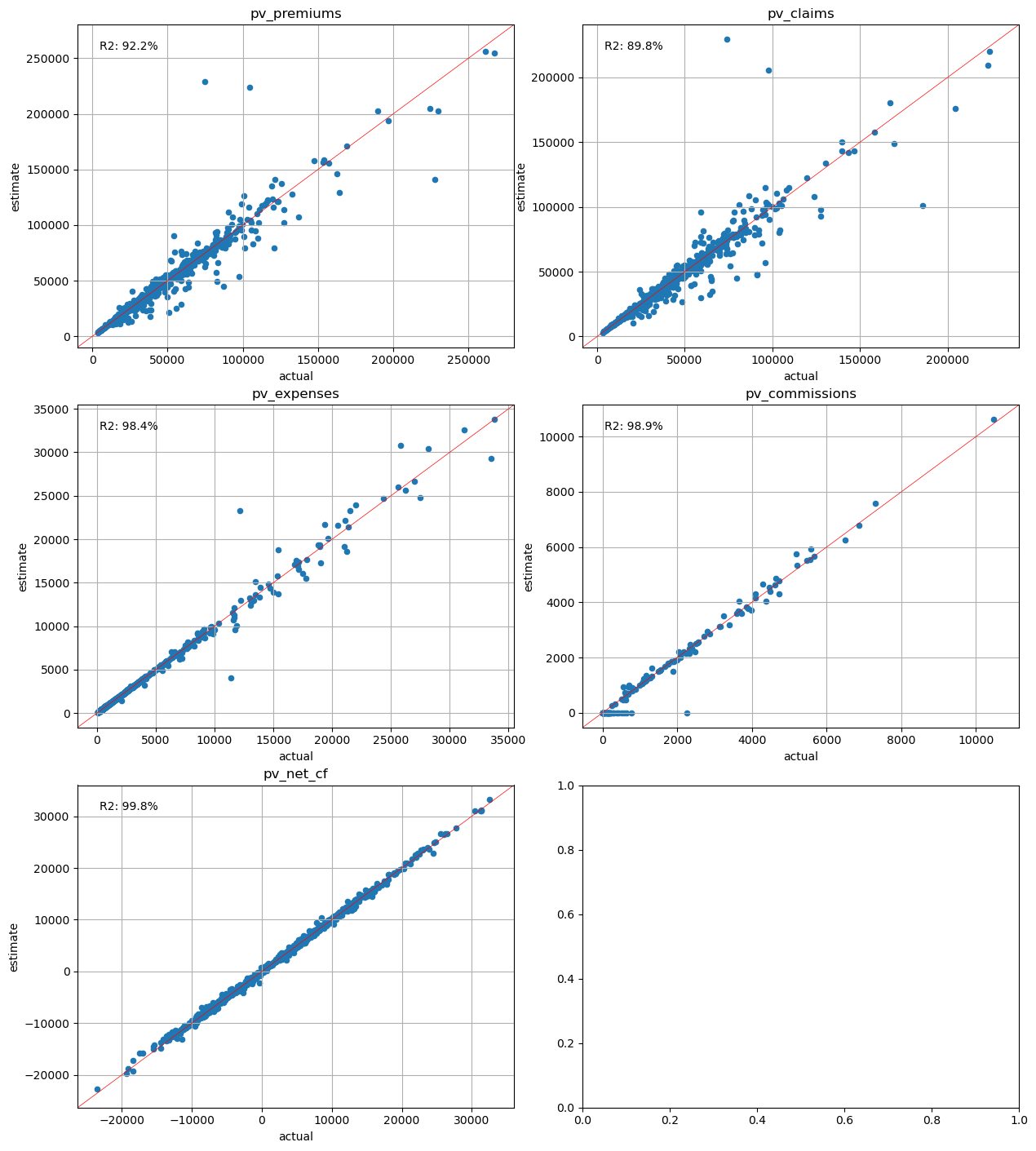
plot_separate_scatter(cluster_cfs.compare(pvs_lapse50), 3, 2)
[20]:
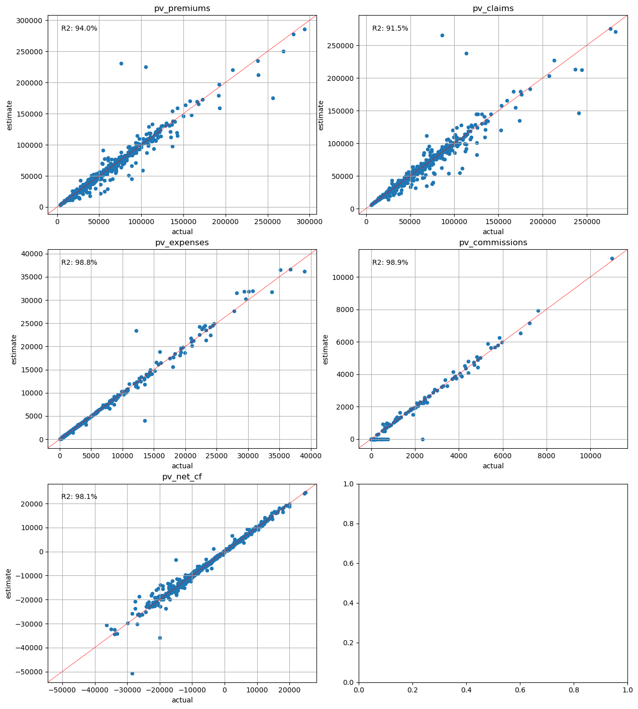
plot_separate_scatter(cluster_cfs.compare(pvs_mort15), 3, 2)
Policy Attribute Calibration#
The next pattern to examine is to use the pollicy attributes as the calibration variables. The attibutes needs to be standardized beforehand. We use the range standardization method based.
Reference
[21]:
loc_vars = (pol_data- pol_data.min()) / (pol_data.max()- pol_data.min())
loc_vars
[21]:
| age_at_entry | policy_term | sum_assured | duration_mth | |
|---|---|---|---|---|
| policy_id | ||||
| 1 | 0.692308 | 0.0 | 0.618182 | 0.113445 |
| 2 | 0.230769 | 1.0 | 0.749495 | 0.890756 |
| 3 | 0.794872 | 0.0 | 0.796970 | 0.159664 |
| 4 | 0.307692 | 1.0 | 0.416162 | 0.584034 |
| 5 | 0.205128 | 0.5 | 0.601010 | 0.315126 |
| ... | ... | ... | ... | ... |
| 9996 | 0.692308 | 1.0 | 0.825253 | 0.701681 |
| 9997 | 0.256410 | 0.5 | 0.824242 | 0.705882 |
| 9998 | 0.641026 | 1.0 | 0.780808 | 0.659664 |
| 9999 | 0.487179 | 1.0 | 0.294949 | 0.168067 |
| 10000 | 0.051282 | 0.5 | 0.571717 | 0.697479 |
10000 rows × 4 columns
[22]:
cluster_attrs = Clusters(loc_vars)
Cashflow Analysis#
[23]:
cluster_attrs.compare_total(cfs)
[23]:
| actual | estimate | error | |
|---|---|---|---|
| 0 | 1.435932e+06 | 1.492568e+06 | 0.039442 |
| 1 | 1.105742e+06 | 1.102142e+06 | -0.003256 |
| 2 | 6.820530e+05 | 6.983101e+05 | 0.023835 |
| 3 | 3.579056e+05 | 3.396505e+05 | -0.051005 |
| 4 | 1.450520e+05 | 1.118500e+05 | -0.228897 |
| 5 | 3.343158e+03 | -6.572615e+03 | -2.965990 |
| 6 | -9.917748e+04 | -1.020972e+05 | 0.029439 |
| 7 | -1.636027e+05 | -1.592419e+05 | -0.026655 |
| 8 | -2.099648e+05 | -2.218798e+05 | 0.056747 |
| 9 | -2.391351e+05 | -2.352241e+05 | -0.016355 |
| 10 | -2.521441e+05 | -2.661291e+05 | 0.055464 |
| 11 | -2.458585e+05 | -2.430511e+05 | -0.011419 |
| 12 | -2.214476e+05 | -2.328187e+05 | 0.051349 |
| 13 | -1.802033e+05 | -1.787738e+05 | -0.007933 |
| 14 | -1.492649e+05 | -1.424064e+05 | -0.045948 |
| 15 | -1.242241e+05 | -1.139114e+05 | -0.083016 |
| 16 | -9.948838e+04 | -9.976519e+04 | 0.002782 |
| 17 | -7.169144e+04 | -7.500936e+04 | 0.046281 |
| 18 | -4.188922e+04 | -4.234964e+04 | 0.010991 |
| 19 | -1.398866e+04 | -9.238264e+03 | -0.339589 |
[24]:
for ax, df, title in zip(generate_subplots(3, (2, 2)), cfs_list, scen_titles):
    plot_cashflows(ax, cluster_attrs.compare_total(df), title)
[25]:
for ax, df, title in zip(generate_subplots(3, (2, 2)), cfs_list, scen_titles):
    plot_colored_scatter(ax, cluster_attrs.compare(df), title=title)
Policy Attribute Analysis#
[26]:
cluster_attrs.compare_total(pol_data, agg=mean_attrs)
[26]:
| actual | estimate | error | |
|---|---|---|---|
| age_at_entry | 3.937720e+01 | 3.939480e+01 | 0.000447 |
| policy_term | 1.493600e+01 | 1.493600e+01 | 0.000000 |
| sum_assured | 5.060517e+09 | 5.060841e+09 | 0.000064 |
| duration_mth | 8.977470e+01 | 8.969640e+01 | -0.000872 |
[27]:
plot_separate_scatter(cluster_attrs.compare(pol_data, agg=mean_attrs), 2, 2)
Present Value Analysis#
[28]:
cluster_attrs.compare_total(pvs)
[28]:
| actual | estimate | error | |
|---|---|---|---|
| pv_premiums | 4.860639e+07 | 4.880437e+07 | 0.004073 |
| pv_claims | 4.331937e+07 | 4.362114e+07 | 0.006966 |
| pv_expenses | 2.949823e+06 | 2.963531e+06 | 0.004647 |
| pv_commissions | 2.748443e+05 | 1.522855e+05 | -0.445921 |
| pv_net_cf | 2.062353e+06 | 2.067409e+06 | 0.002452 |
[29]:
cluster_attrs.compare_total(pvs_lapse50)
[29]:
| actual | estimate | error | |
|---|---|---|---|
| pv_premiums | 4.280459e+07 | 4.303844e+07 | 0.005463 |
| pv_claims | 3.831786e+07 | 3.863643e+07 | 0.008314 |
| pv_expenses | 2.579405e+06 | 2.593662e+06 | 0.005527 |
| pv_commissions | 2.653036e+05 | 1.478034e+05 | -0.442890 |
| pv_net_cf | 1.642024e+06 | 1.660543e+06 | 0.011278 |
[30]:
cluster_attrs.compare_total(pvs_mort15)
[30]:
| actual | estimate | error | |
|---|---|---|---|
| pv_premiums | 4.853083e+07 | 4.872875e+07 | 0.004078 |
| pv_claims | 4.973258e+07 | 5.007948e+07 | 0.006975 |
| pv_expenses | 2.946908e+06 | 2.960610e+06 | 0.004649 |
| pv_commissions | 2.748356e+05 | 1.522817e+05 | -0.445917 |
| pv_net_cf | -4.423494e+06 | -4.463622e+06 | 0.009072 |
[31]:
plot_separate_scatter(cluster_attrs.compare(pvs), 3, 2)
[32]:
plot_separate_scatter(cluster_attrs.compare(pvs_lapse50), 3, 2)
[33]:
plot_separate_scatter(cluster_attrs.compare(pvs_mort15), 3, 2)
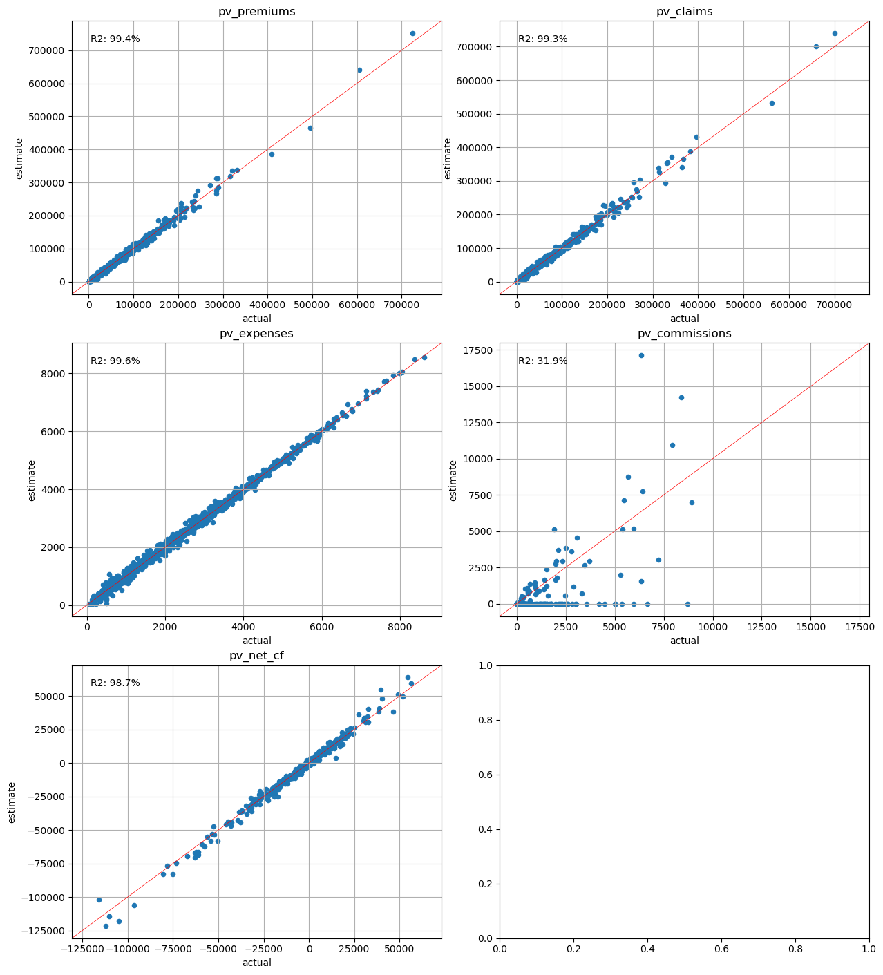
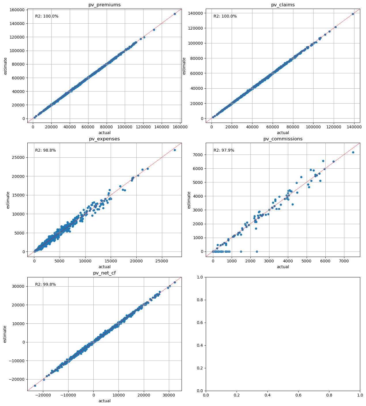
Present Value Calibration#
The last approach is to use the present values of cashflows for the variables. This approach makes sense as present values are most often the final figures to be reported.
[34]:
cluster_pvs = Clusters(pvs)
Cashflow Analysis#
[35]:
cluster_pvs.compare_total(cfs)
[35]:
| actual | estimate | error | |
|---|---|---|---|
| 0 | 1.435932e+06 | 1.457022e+06 | 0.014687 |
| 1 | 1.105742e+06 | 1.063551e+06 | -0.038157 |
| 2 | 6.820530e+05 | 6.741228e+05 | -0.011627 |
| 3 | 3.579056e+05 | 3.501045e+05 | -0.021797 |
| 4 | 1.450520e+05 | 1.686178e+05 | 0.162465 |
| 5 | 3.343158e+03 | 2.877806e+04 | 7.608045 |
| 6 | -9.917748e+04 | -8.496205e+04 | -0.143333 |
| 7 | -1.636027e+05 | -1.547262e+05 | -0.054257 |
| 8 | -2.099648e+05 | -1.954995e+05 | -0.068894 |
| 9 | -2.391351e+05 | -2.431312e+05 | 0.016711 |
| 10 | -2.521441e+05 | -2.689157e+05 | 0.066516 |
| 11 | -2.458585e+05 | -2.475185e+05 | 0.006752 |
| 12 | -2.214476e+05 | -2.214978e+05 | 0.000227 |
| 13 | -1.802033e+05 | -1.929181e+05 | 0.070558 |
| 14 | -1.492649e+05 | -1.585572e+05 | 0.062254 |
| 15 | -1.242241e+05 | -1.226541e+05 | -0.012638 |
| 16 | -9.948838e+04 | -1.001879e+05 | 0.007031 |
| 17 | -7.169144e+04 | -6.581462e+04 | -0.081974 |
| 18 | -4.188922e+04 | -3.618109e+04 | -0.136267 |
| 19 | -1.398866e+04 | -1.110348e+04 | -0.206252 |
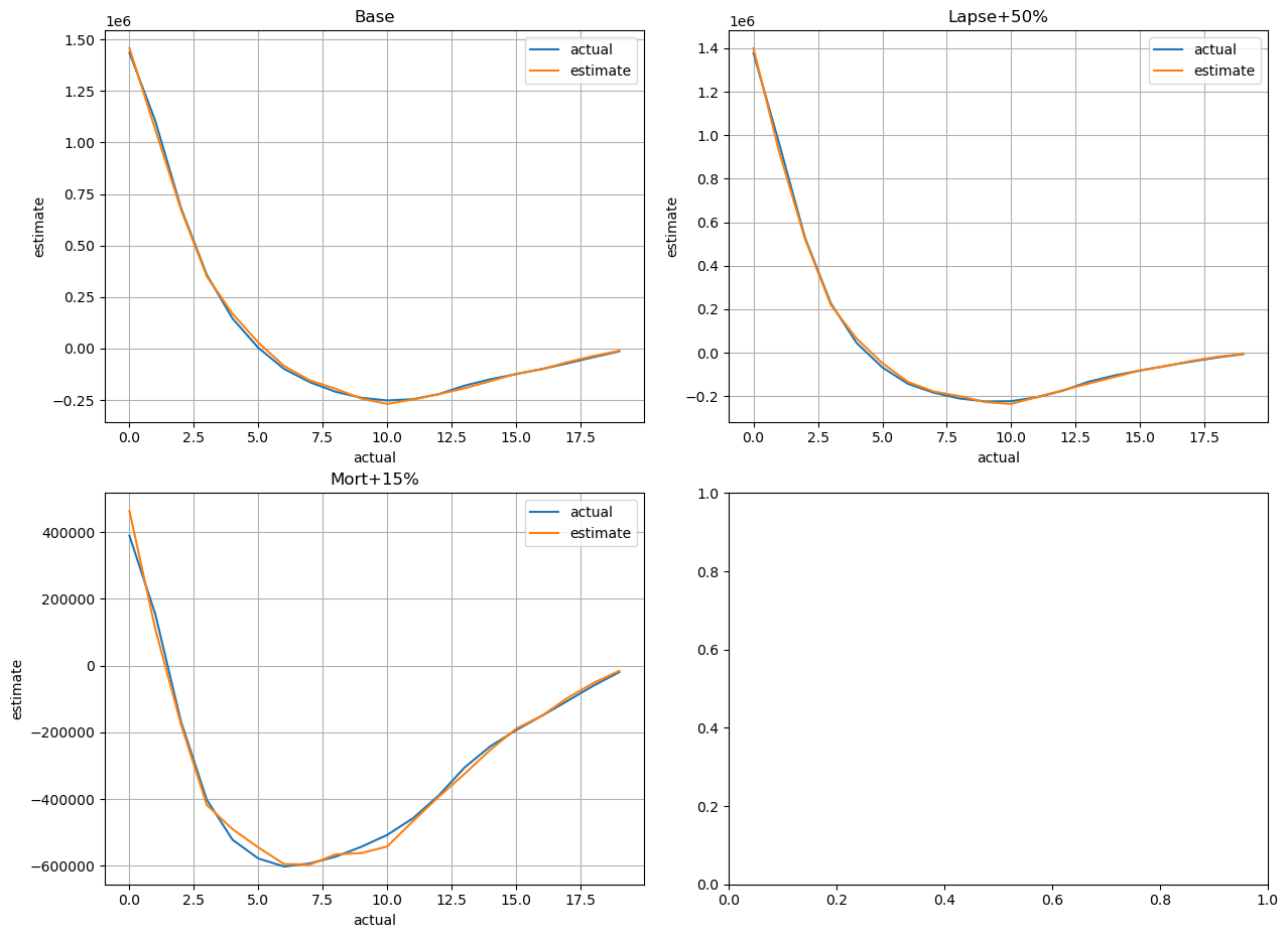
[36]:
for ax, df, title in zip(generate_subplots(3, (2, 2)), cfs_list, scen_titles):
    plot_cashflows(ax, cluster_pvs.compare_total(df), title)
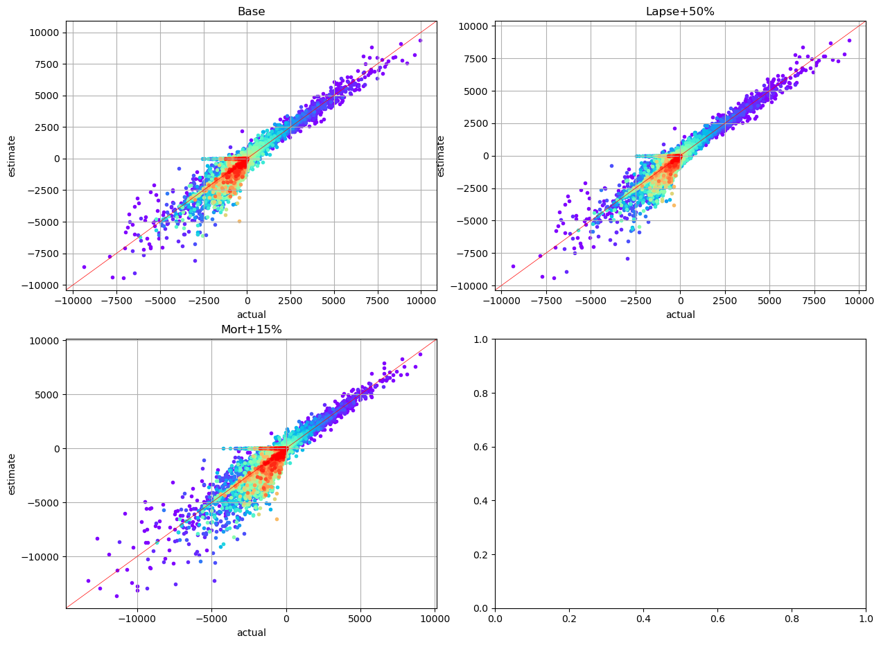
[37]:
for ax, df, title in zip(generate_subplots(3, (2, 2)), cfs_list, scen_titles):
    plot_colored_scatter(ax, cluster_pvs.compare(df), title=title)
Policy Attribute Analysis#
[38]:
cluster_pvs.compare_total(pol_data, agg=mean_attrs)
[38]:
| actual | estimate | error | |
|---|---|---|---|
| age_at_entry | 3.937720e+01 | 3.908320e+01 | -0.007466 |
| policy_term | 1.493600e+01 | 1.491800e+01 | -0.001205 |
| sum_assured | 5.060517e+09 | 4.848571e+09 | -0.041882 |
| duration_mth | 8.977470e+01 | 9.025770e+01 | 0.005380 |
[39]:
plot_separate_scatter(cluster_pvs.compare(pol_data, agg=mean_attrs), 2, 2)
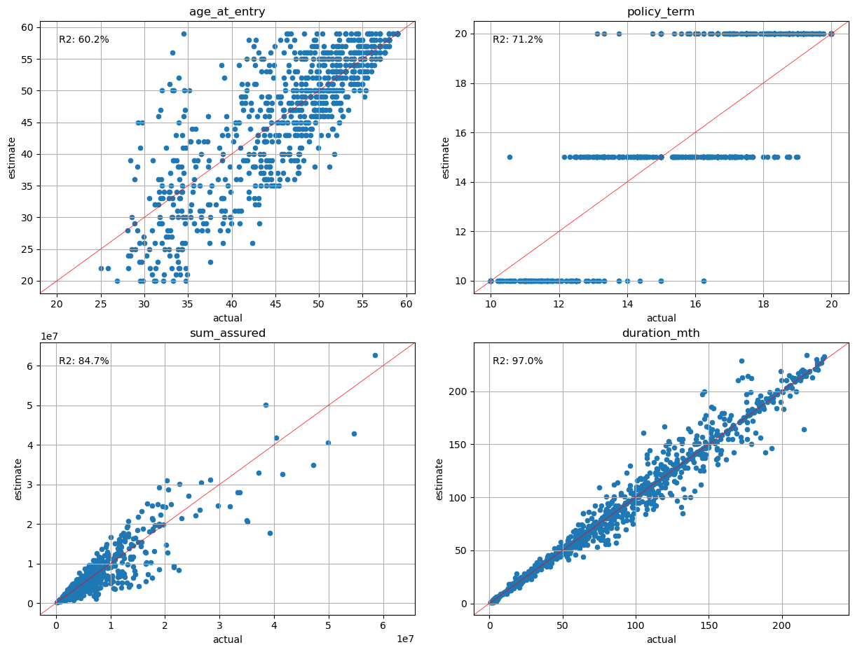
Present Value Analysis#
[40]:
cluster_pvs.compare_total(pvs)
[40]:
| actual | estimate | error | |
|---|---|---|---|
| pv_premiums | 4.860639e+07 | 4.860263e+07 | -0.000077 |
| pv_claims | 4.331937e+07 | 4.329537e+07 | -0.000554 |
| pv_expenses | 2.949823e+06 | 2.967432e+06 | 0.005970 |
| pv_commissions | 2.748443e+05 | 2.609099e+05 | -0.050699 |
| pv_net_cf | 2.062353e+06 | 2.078910e+06 | 0.008029 |
[41]:
cluster_pvs.compare_total(pvs_lapse50)
[41]:
| actual | estimate | error | |
|---|---|---|---|
| pv_premiums | 4.280459e+07 | 4.279176e+07 | -0.000300 |
| pv_claims | 3.831786e+07 | 3.828253e+07 | -0.000922 |
| pv_expenses | 2.579405e+06 | 2.604033e+06 | 0.009548 |
| pv_commissions | 2.653036e+05 | 2.518241e+05 | -0.050808 |
| pv_net_cf | 1.642024e+06 | 1.653374e+06 | 0.006912 |
[42]:
cluster_pvs.compare_total(pvs_mort15)
[42]:
| actual | estimate | error | |
|---|---|---|---|
| pv_premiums | 4.853083e+07 | 4.852611e+07 | -0.000097 |
| pv_claims | 4.973258e+07 | 4.970372e+07 | -0.000580 |
| pv_expenses | 2.946908e+06 | 2.964534e+06 | 0.005981 |
| pv_commissions | 2.748356e+05 | 2.609015e+05 | -0.050700 |
| pv_net_cf | -4.423494e+06 | -4.403046e+06 | -0.004623 |
[43]:
plot_separate_scatter(cluster_pvs.compare(pvs), 3, 2)
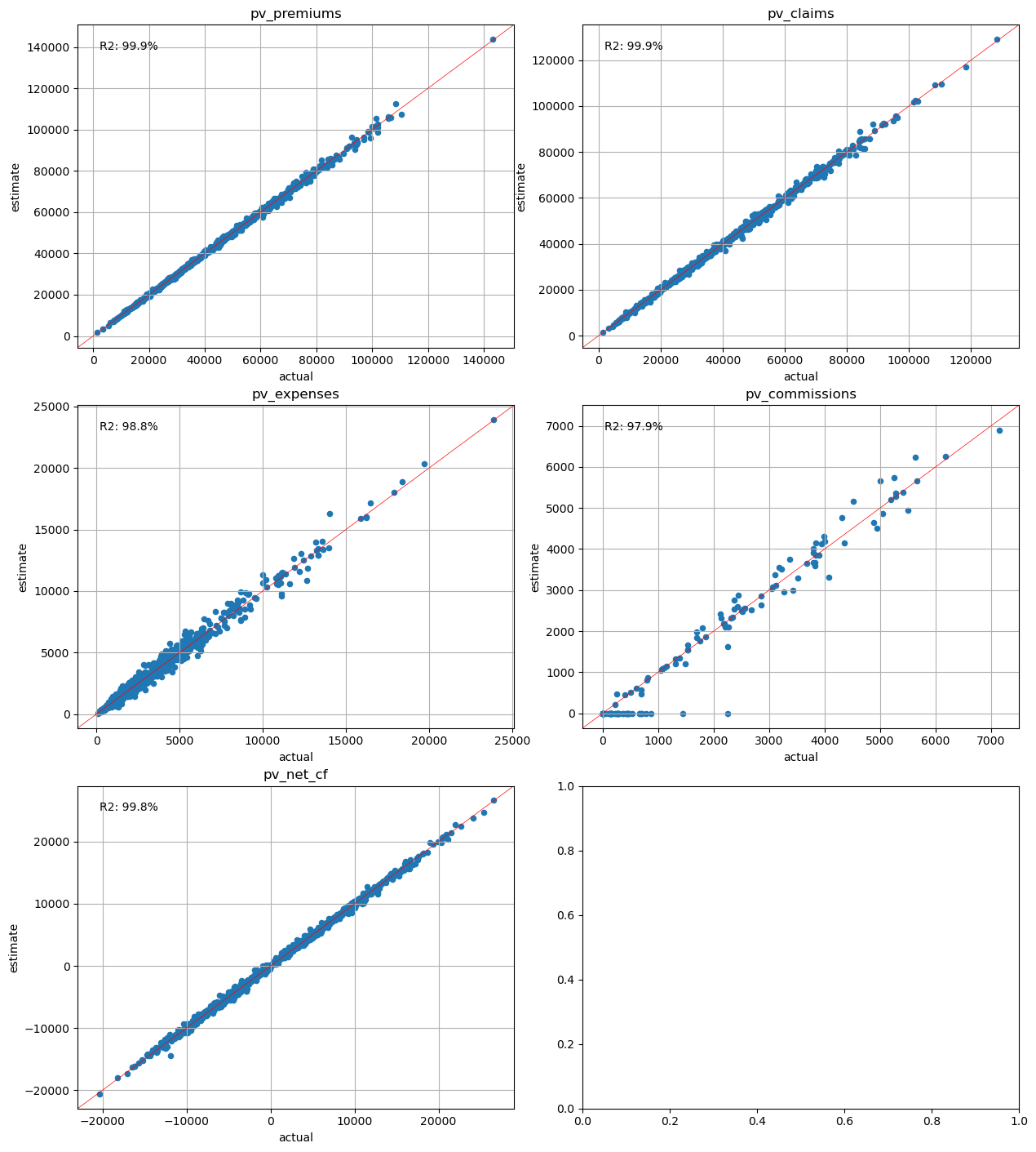
[44]:
plot_separate_scatter(cluster_pvs.compare(pvs_lapse50), 3, 2)
[45]:
plot_separate_scatter(cluster_pvs.compare(pvs_mort15), 3, 2)
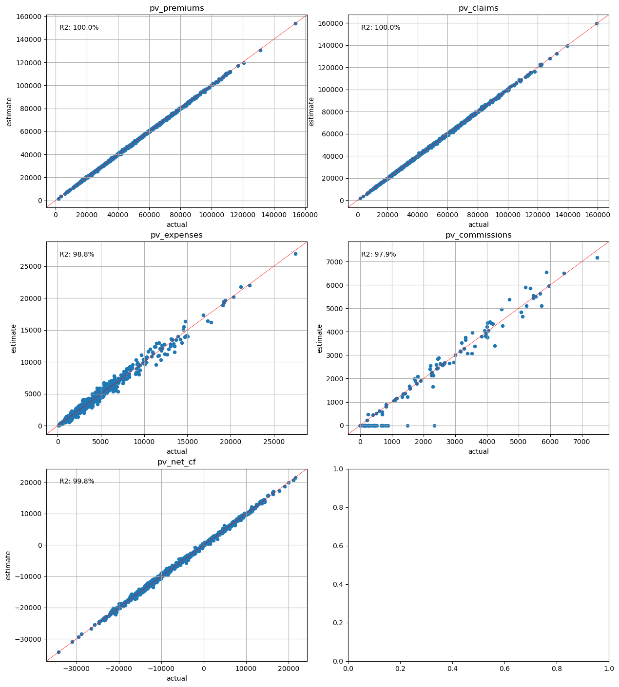
Conclustion#
As expected, the results are highly dependent on the choice of calibration variables. The variables chosen for calibration are more accurately estimated by the proxy portfolio than others. In practice, the present values of cashflows are often the most important metrics. Our exercise shows that choosing the present values of net cashflows for the variables estimates the seriatim results best, with error percentages below 1% in all the scenarios.