G2PP#
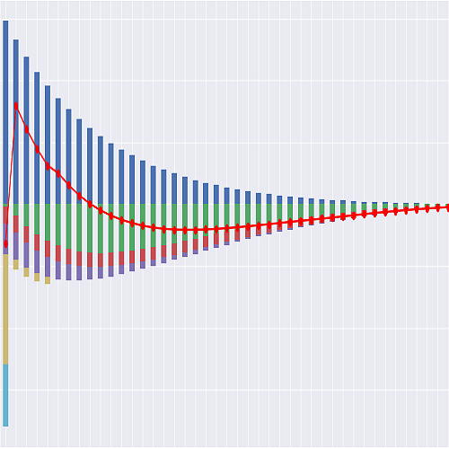
Monthly G2++ interest rate scenarios fitted to an initial curve.
The two-additive-factor Gaussian model G2++ (Brigo and Mercurio, 2nd ed. 2006, section 4.2) under the risk-neutral measure:
with \(x(0) = y(0) = 0\) and \(\varphi\) fitted exactly to the initial curve
\(P^M(0, t)\). Each month, \(x\), \(y\) and \(\int (x + y) du\) are drawn
together from their exact Gaussian transition (cov_step()), so the deflators
reproduce the initial curve up to Monte Carlo noise. Time is in years, and month i is
\(t_i = i/12\) (t_()). N is scen_size() and n is step_size().
Inputs are read at run time from the Excel file input_file, located next to
the model folder: sheet Params (G2++ parameters and run settings), sheet Curve
(initial spot rates by maturity, one column per curve ID) and sheet Fund (shares of
bond funds by years to maturity). The initial curve is not extrapolated, so it must reach
every maturity a run needs. After editing the file in place, call clear_all() on the
model; assigning another input_file recalculates automatically.
Outputs for liability models are arrays with one row per scenario. Row 0 is the
certainty-equivalent (CE) scenario, which follows the initial forward curve, and row k
is stochastic scenario k (see scen_index()):
disc_factor_paths(): deflators \(D(t_i)\), for discounting cash flows at \(t_i\)fund_return_paths(): returns over \([t_i, t_{i+1})\) of the bond fund chosen byfund_id()bank_return_paths(): bank-account returns over \([t_i, t_{i+1})\)short_rate_paths(),spot_rate_paths(): short rates and yields
- input_file#
Name of the Excel input file, relative to the folder that contains the model folder, or an absolute path.
"g2pp_input.xlsx"by default.
- dt#
Length of a monthly step in years, 1/12.
- np#
The numpy module.
- pd#
The pandas module.
See also
Damiano Brigo, Fabio Mercurio (2001, 2nd Ed. 2006). Interest Rate Models - Theory and Practice with Smile, Inflation and Credit
Cells
|
\(B_a(t_i, t_j) = (1 - e^{-a(t_j - t_i)})/a\), the loading of \(x(t_i)\) in \(\ln P(t_i, t_j)\) |
|
\(B_b(t_i, t_j) = (1 - e^{-b(t_j - t_i)})/b\), the loading of \(y(t_i)\) in \(\ln P(t_i, t_j)\) |
|
Expected short rates \(E[r(t_i)] = \varphi(t_i)\) for i = 0 to n |
|
Zero-coupon bond price \(P(t_i, t_j)\) by scenario |
|
Variance \(V(t_i, t_j)\) of \(\int_{t_i}^{t_j} (x(u) + y(u)) du\) given \(\mathcal{F}_{t_i}\) |
|
Variances of the short rates \(r(t_i)\) for i = 0 to n |
|
Mean reversion speed \(a\) of \(x(t)\), from the |
|
Integrated factors \(A(t_i) = \int_0^{t_i}(x(u) + y(u))du\) by scenario |
Whether antithetic variates are used, from the |
|
|
Mean reversion speed \(b\) of \(y(t)\), from the |
Bank-account return \(R_i = D(t_i)/D(t_{i+1}) - 1\) over \([t_i, t_{i+1})\) by scenario |
|
Bank-account returns over \([t_i, t_{i+1})\) for every scenario and month |
|
Bank-account return of the CE scenario, the one-month forward \(P^M(0, t_i)/P^M(0, t_{i+1}) - 1\) |
|
Deflator of the CE scenario, \(P^M(0, t_i)\) |
|
Short rate of the CE scenario, the initial forward \(f^M(0, t_i)\) |
|
|
Annually compounded m-month yield at \(t_i\) in the CE scenario, \((P^M(0, t_i)/P^M(0, t_{i+m}))^{12/m} - 1\) |
Square root \(L\) of |
|
Compounding of the input spot rates, |
|
|
Covariance \(C\) of one exact monthly step |
|
Column of the |
Knots of the selected initial curve |
|
Spot rates from the |
|
|
Deflator \(D(t_i)\), the reciprocal of the bank account, by scenario |
Deflators \(D(t_i)\) for every scenario and month |
|
|
Volatility \(\eta\) of \(y(t)\), from the |
Shares of the selected fund in zero-coupon bonds, by maturity in months |
|
Share of the selected fund held in the bank account (0 if it has no cash row) |
|
|
Column of the |
|
Variance \(s^2\) of \(\ln(AV(t_j)/AV_0)\) for the selected fund |
Market-value return \(R^F_i\) of the selected fund over \([t_i, t_{i+1})\), by scenario |
|
Returns of the selected fund over \([t_i, t_{i+1})\) for every scenario and month |
|
Fund shares from the |
|
Path of the Excel input file |
|
|
Initial instantaneous forward rate \(f^M(0, t_i)\) |
|
Initial discount factor \(P^M(0, t_i)\) |
Validated values from the |
|
|
Deterministic shift \(\varphi(t_i)\) that fits the model to the initial curve |
|
Correlation \(\rho\) of \(W_1\) and \(W_2\), from the |
Scenario IDs 0 to N, where 0 is the CE scenario |
|
Number of stochastic scenarios N, from the |
|
Deflators, returns and short rates for every scenario and month, in long format |
|
|
Seed of the random number generator, from the |
|
Correlated shocks \((\varepsilon_1, \varepsilon_2, \varepsilon_3)\) of the step from month i to i+1 |
|
Short rate \(r(t_i) = x(t_i) + y(t_i) + \varphi(t_i)\) by scenario |
Short rates \(r(t_i)\) for every scenario and month |
|
|
Volatility \(\sigma\) of \(x(t)\), from the |
|
Annually compounded m-month yield at \(t_i\), \(P(t_i, t_{i+m})^{-12/m} - 1\), by scenario |
Annually compounded m-month yields for every scenario and month |
|
Standard normal random numbers for all steps and scenarios |
|
Number of monthly steps n, from the |
|
|
k-year par rate at \(t_i\) with an annual fixed leg, by scenario |
|
Time \(t_i = i/12\) in years of month |
|
Factor \(x(t_i)\) by scenario |
|
Factor \(y(t_i)\) by scenario |
|
Return over \([t_i, t_{i+1})\) of a zero-coupon bond with m months to maturity at \(t_i\), by scenario |
- input_path()[source]#
Path of the Excel input file
input_fileresolved against the folder that contains the model folder, so the defaultg2pp_input.xlsxsits next toBasicG2PP/. An absoluteinput_fileis used as it is.- Returns:
pathlib.Path
- param_table()[source]#
Validated values from the
ParamssheetReads the
Paramssheet (columnsparameter,valueanddescription) ofinput_path(), converts each value to its type and checks it. RaisesValueErrorlisting every problem: a missing value or one of the wrong type,a,borsigmanot positive,etanegative,rhooutside [-1, 1], sizes below 1, a negative seed, an oddscen_sizewithantitheticon, or acompoundingother thanannualorcontinuous.- Returns:
pandas.Series indexed by parameter name, with object dtype (values are float, int, bool or str)
- curve_table()[source]#
Spot rates from the
CurvesheetColumn
maturityholds maturities in years and every other column is a curve, named by its curve ID. A curve ends at its last non-blank row. RaisesValueErrorfor maturities that are not positive and increasing, or a blank inside a curve.- Returns:
pandas.DataFrame indexed by
maturity(years), one float column per curve ID
- fund_table()[source]#
Fund shares from the
FundsheetColumn
maturityholds the years to maturity of zero-coupon bonds (a whole number of months), orcashfor the bank account. Every other column is a fund, named by its fund ID, holding its shares; a blank share is 0. RaisesValueErrorfor a maturity that is neithercashnor a positive whole number of months, a repeated maturity, a negative share, or a fund whose shares do not sum to 1 within 1e-9.- Returns:
pandas.DataFrame indexed by
maturity("cash"or years), one float column per fund ID
- step_size()[source]#
Number of monthly steps n, from the
ParamssheetThe projection runs from month 0 to month n, so \(t_n\) = n/12 years must not be later than the last maturity of the curve.
- antithetic()[source]#
Whether antithetic variates are used, from the
ParamssheetIf
True, stochastic scenario k + N/2 uses the negated random numbers of scenario k. Seestd_norm_rand().
- curve_knots()[source]#
Knots of the selected initial curve
The maturities \(t_k\) of the curve
curve_id()and the log discount factors \(\ln P^M(0, t_k) = -t_k \ln(1 + s_k)\) for annually compounded spot rates \(s_k\), or \(-t_k s_k\) for continuously compounded ones. Both arrays start with the knot \(t = 0\), \(\ln P^M(0, 0) = 0\).Raises
ValueErrorifcurve_id()is not a column of theCurvesheet, or if the curve ends before the projection horizon \(t_n\). The curve is not extrapolated.- Returns:
knot times and log discount factors
- Return type:
tuple of two 1-D numpy arrays of equal length
- mkt_zcb(i)[source]#
Initial discount factor \(P^M(0, t_i)\)
\(\ln P^M(0, t)\) is interpolated linearly in \(t\) between the knots of
curve_knots(), so instantaneous forwards are flat between knots. RaisesValueErrorfor \(t_i\) past the last maturity: the curve is not extrapolated.
- mkt_fwd(i)[source]#
Initial instantaneous forward rate \(f^M(0, t_i)\)
The flat forward of the knot interval \([t_k, t_{k+1})\) that contains \(t_i\), and of the last interval at the final knot, so no curve beyond \(t_i\) is needed:
\[f^M(0, t_i) = \frac{\ln P^M(0, t_k) - \ln P^M(0, t_{k+1})}{t_{k+1} - t_k}\]
- Ba_t_T(i, j)[source]#
\(B_a(t_i, t_j) = (1 - e^{-a(t_j - t_i)})/a\), the loading of \(x(t_i)\) in \(\ln P(t_i, t_j)\)
- Bb_t_T(i, j)[source]#
\(B_b(t_i, t_j) = (1 - e^{-b(t_j - t_i)})/b\), the loading of \(y(t_i)\) in \(\ln P(t_i, t_j)\)
- V_t_T(i, j)[source]#
Variance \(V(t_i, t_j)\) of \(\int_{t_i}^{t_j} (x(u) + y(u)) du\) given \(\mathcal{F}_{t_i}\)
With \(\tau = t_j - t_i\) (Brigo and Mercurio, section 4.2):
\[V(t, T) = \frac{\sigma^2}{a^2}\left[\tau + \frac{2}{a}e^{-a\tau} - \frac{1}{2a}e^{-2a\tau} - \frac{3}{2a}\right] + \frac{\eta^2}{b^2}\left[\tau + \frac{2}{b}e^{-b\tau} - \frac{1}{2b}e^{-2b\tau} - \frac{3}{2b}\right] + \frac{2\rho\sigma\eta}{ab}\left[\tau + \frac{e^{-a\tau} - 1}{a} + \frac{e^{-b\tau} - 1}{b} - \frac{e^{-(a+b)\tau} - 1}{a + b}\right]\]Computed with
expm1, which keeps the digits that \(e^{-a\tau} - 1\) loses for small \(\tau\).
- phi(i)[source]#
Deterministic shift \(\varphi(t_i)\) that fits the model to the initial curve
\[\varphi(t) = f^M(0, t) + \frac{\sigma^2}{2a^2}(1 - e^{-at})^2 + \frac{\eta^2}{2b^2}(1 - e^{-bt})^2 + \frac{\rho\sigma\eta}{ab}(1 - e^{-at})(1 - e^{-bt})\]
- E_rt()[source]#
Expected short rates \(E[r(t_i)] = \varphi(t_i)\) for i = 0 to n
- Returns:
numpy array of shape (n+1,)
- Var_rt()[source]#
Variances of the short rates \(r(t_i)\) for i = 0 to n
\[\mathrm{Var}[r(t)] = \frac{\sigma^2}{2a}(1 - e^{-2at}) + \frac{\eta^2}{2b}(1 - e^{-2bt}) + \frac{2\rho\sigma\eta}{a + b}(1 - e^{-(a+b)t})\]- Returns:
numpy array of shape (n+1,)
- fund_logvar(j)[source]#
Variance \(s^2\) of \(\ln(AV(t_j)/AV_0)\) for the selected fund
Used by the closed-form GMAB value of CashValue_ME_G2PP,
formula_gmab_g2pp(). For an all-cash fund, \(AV(t_j)/AV_0 = 1/D(t_j)\) and \(s^2 = V(0, t_j)\). For a fund that holds a single maturity \(\tau\), the monthly log return is linear in \(x\) and \(y\) (seezcb_return_mth()), and \(s^2\) follows from a covariance recursion for \((x, y, \ln AV)\) over the months. RaisesValueErrorfor other funds, which have no exact closed form.
- std_norm_rand()[source]#
Standard normal random numbers for all steps and scenarios
Drawn by
numpy.random.default_rng(seed())in step-major order, so a longer projection leaves earlier months unchanged. Withantithetic(), the first N/2 scenarios are drawn and the rest are their negatives.- Returns:
numpy array of shape (n, N, 3)
- cov_step()[source]#
Covariance \(C\) of one exact monthly step
The covariance of \(x(t+\Delta)\), \(y(t+\Delta)\) and \(\int_t^{t+\Delta}(x + y)du\) given \(\mathcal{F}_t\), with \(\Delta\) =
dt. It does not depend on \(t\):\[ \begin{align}\begin{aligned}C_{11} = \frac{\sigma^2}{2a}(1 - e^{-2a\Delta}), \quad C_{22} = \frac{\eta^2}{2b}(1 - e^{-2b\Delta}), \quad C_{12} = \frac{\rho\sigma\eta}{a + b}(1 - e^{-(a+b)\Delta})\\C_{13} = \frac{\sigma^2}{2a^2}(1 - e^{-a\Delta})^2 + \frac{\rho\sigma\eta}{b}\left[\frac{1 - e^{-a\Delta}}{a} - \frac{1 - e^{-(a+b)\Delta}}{a + b}\right]\\C_{23} = \frac{\eta^2}{2b^2}(1 - e^{-b\Delta})^2 + \frac{\rho\sigma\eta}{a}\left[\frac{1 - e^{-b\Delta}}{b} - \frac{1 - e^{-(a+b)\Delta}}{a + b}\right]\\C_{33} = V(t, t + \Delta)\end{aligned}\end{align} \]- Returns:
numpy array of shape (3, 3)
- chol_step()[source]#
Square root \(L\) of
cov_step(), with \(LL^T = C\)The Cholesky factor, or a symmetric square root from
numpy.linalg.eighwhen \(C\) is singular, for example when \(\eta = 0\).- Returns:
numpy array of shape (3, 3)
- shocks(i)[source]#
Correlated shocks \((\varepsilon_1, \varepsilon_2, \varepsilon_3)\) of the step from month i to i+1
\(\varepsilon = L z\) with \(L\) =
chol_step()and \(z\) the random numbers ofstd_norm_rand()for step i.- Returns:
numpy array of shape (N, 3)
- x(i)[source]#
Factor \(x(t_i)\) by scenario
\(x(0) = 0\) and \(x(t_{i+1}) = x(t_i)e^{-a\Delta} + \varepsilon_1\).
- Returns:
numpy array of shape (N,)
- y(i)[source]#
Factor \(y(t_i)\) by scenario
\(y(0) = 0\) and \(y(t_{i+1}) = y(t_i)e^{-b\Delta} + \varepsilon_2\).
- Returns:
numpy array of shape (N,)
- accum_xy(i)[source]#
Integrated factors \(A(t_i) = \int_0^{t_i}(x(u) + y(u))du\) by scenario
\(A(t_{i+1}) = A(t_i) + B_a(\Delta)x(t_i) + B_b(\Delta)y(t_i) + \varepsilon_3\), which is exact for the monthly step.
- Returns:
numpy array of shape (N,)
- short_rate(i)[source]#
Short rate \(r(t_i) = x(t_i) + y(t_i) + \varphi(t_i)\) by scenario
- Returns:
numpy array of shape (N,)
- disc_factor(i)[source]#
Deflator \(D(t_i)\), the reciprocal of the bank account, by scenario
\[D(t_i) = P^M(0, t_i)\exp\left(-\tfrac{1}{2}V(0, t_i) - A(t_i)\right)\]so that \(E[D(t_i)] = P^M(0, t_i)\).
- Returns:
numpy array of shape (N,)
- bank_return_mth(i)[source]#
Bank-account return \(R_i = D(t_i)/D(t_{i+1}) - 1\) over \([t_i, t_{i+1})\) by scenario
- Returns:
numpy array of shape (N,)
- P_t_T(i, j)[source]#
Zero-coupon bond price \(P(t_i, t_j)\) by scenario
\[P(t, T) = \frac{P^M(0, T)}{P^M(0, t)} \exp\left(\tfrac{1}{2}[V(t, T) - V(0, T) + V(0, t)] - B_a(t, T)x(t) - B_b(t, T)y(t)\right)\]Needs the curve out to \(t_j\).
- Returns:
numpy array of shape (N,)
- spot_rate(i, m)[source]#
Annually compounded m-month yield at \(t_i\), \(P(t_i, t_{i+m})^{-12/m} - 1\), by scenario
- Returns:
numpy array of shape (N,)
- swap_rate(i, k)[source]#
k-year par rate at \(t_i\) with an annual fixed leg, by scenario
\[\frac{1 - P(t_i, t_i + k)}{\sum_{l=1}^{k} P(t_i, t_i + l)}\]- Returns:
numpy array of shape (N,)
- ce_bank_return_mth(i)[source]#
Bank-account return of the CE scenario, the one-month forward \(P^M(0, t_i)/P^M(0, t_{i+1}) - 1\)
- ce_spot_rate(i, m)[source]#
Annually compounded m-month yield at \(t_i\) in the CE scenario, \((P^M(0, t_i)/P^M(0, t_{i+m}))^{12/m} - 1\)
Share of the selected fund held in the bank account (0 if it has no cash row)
Shares of the selected fund in zero-coupon bonds, by maturity in months
Bonds with a zero share are left out.
- Returns:
pandas.Series of floats indexed by maturity in months (int)
- zcb_return_mth(i, m)[source]#
Return over \([t_i, t_{i+1})\) of a zero-coupon bond with m months to maturity at \(t_i\), by scenario
The bond is bought at \(t_i\) and sold a month later. With \(T = t_{i+m}\):
\[\ln\frac{P(t_{i+1}, T)}{P(t_i, T)} = \ln P^M(0, t_i) - \ln P^M(0, t_{i+1}) + \tfrac{1}{2}[V(t_{i+1}, T) - V(t_i, T) + V(0, t_{i+1}) - V(0, t_i)] - B_a(t_{i+1}, T)x(t_{i+1}) - B_b(t_{i+1}, T)y(t_{i+1}) + B_a(t_i, T)x(t_i) + B_b(t_i, T)y(t_i)\]\(P^M(0, T)\) cancels, so the return needs the curve only up to \(t_{i+1}\).
- Returns:
numpy array of shape (N,)
- fund_return_mth(i)[source]#
Market-value return \(R^F_i\) of the selected fund over \([t_i, t_{i+1})\), by scenario
The fund holds the bank account and zero-coupon bonds in the shares of
fund_cash_share()andfund_bond_shares(), sells the bonds after a month and rebalances to the same shares:\[R^F_i = w_c R_i + \sum_m w_m \left[\frac{P(t_{i+1}, t_{i+m})}{P(t_i, t_{i+m})} - 1\right]\]- Returns:
numpy array of shape (N,)
- scen_index()[source]#
Scenario IDs 0 to N, where 0 is the CE scenario
- Returns:
pandas.RangeIndex named
scen_id
- disc_factor_paths()[source]#
Deflators \(D(t_i)\) for every scenario and month
- Returns:
numpy array of shape (N+1, n+1); row 0 is the CE scenario
- bank_return_paths()[source]#
Bank-account returns over \([t_i, t_{i+1})\) for every scenario and month
- Returns:
numpy array of shape (N+1, n); row 0 is the CE scenario
- fund_return_paths()[source]#
Returns of the selected fund over \([t_i, t_{i+1})\) for every scenario and month
In the CE scenario every bond earns the one-month forward, so row 0 is the CE bank-account return whatever the fund’s shares.
- Returns:
numpy array of shape (N+1, n); row 0 is the CE scenario
- short_rate_paths()[source]#
Short rates \(r(t_i)\) for every scenario and month
- Returns:
numpy array of shape (N+1, n+1); row 0 is the CE scenario
- spot_rate_paths(m)[source]#
Annually compounded m-month yields for every scenario and month
Needs the curve out to \(t_{n+m}\).
- Returns:
numpy array of shape (N+1, n+1); row 0 is the CE scenario
- scenario_table()[source]#
Deflators, returns and short rates for every scenario and month, in long format
For inspection and export to CSV or npz. The returns over the month after \(t_n\) are NaN.
- Returns:
pandas.DataFrame indexed by (
scen_id,t) with columnsdisc_factor,bank_return_mth,fund_return_mthandshort_rate
- t_(i)#
Time \(t_i = i/12\) in years of month
i