Note
Go to the end to download the full example code.
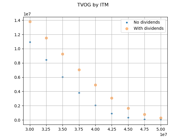
Black-Scholes-Merton on dividend paying stock#
As the 2. Extended Stochastic Example shows, time values of options and guarantees on a GMAB policy can be calculated using the Black-Scholes-Merton formula on a dividend paying stock, when maintenance fees are deducted from account value at a constant rate, by regarding the fees as dividends.
The Black-Scholes-Merton pricing formula for European put options on a dividend paying stock can be expressed as below, where \(X\), \(S_{0}\), \(q\) correspond to the sum assured, the initial account value and the maintenence fee rate(1%) in this example.
The graph below compares the option values with the maintenance fee deduction against the corresponding values without fee deduction for various in-the-moneyness.
Reference: Options, Futures, and Other Derivatives by John C.Hull
See also
1. Simple Stochastic Example notebook in the
savingslibrary2. Extended Stochastic Example notebook in the
savingslibrary
import modelx as mx
import pandas as pd
import matplotlib.pyplot as plt
from scipy.stats import norm, lognorm
import numpy as np

ex1 = mx.read_model("CashValue_ME_EX1").Projection
ex2 = mx.read_model("CashValue_ME_EX2").Projection

ex1.model_point_table = ex1.model_point_moneyness
ex2.model_point_table = ex2.model_point_moneyness
S0 = ex1.model_point_table['premium_pp'] * ex1.model_point_table['policy_count']

fig, ax = plt.subplots()
ax.scatter(S0, ex1.formula_option_put(120), s= 10, alpha=1, label='No dividends')
ax.scatter(S0, ex2.formula_option_put(120), alpha=0.5, label='With dividends')
ax.legend()
ax.grid(True)
fig.suptitle('TVOG by ITM')

ex1.model.close()
ex2.model.close()
Total running time of the script: (0 minutes 1.451 seconds)