Account value distribution

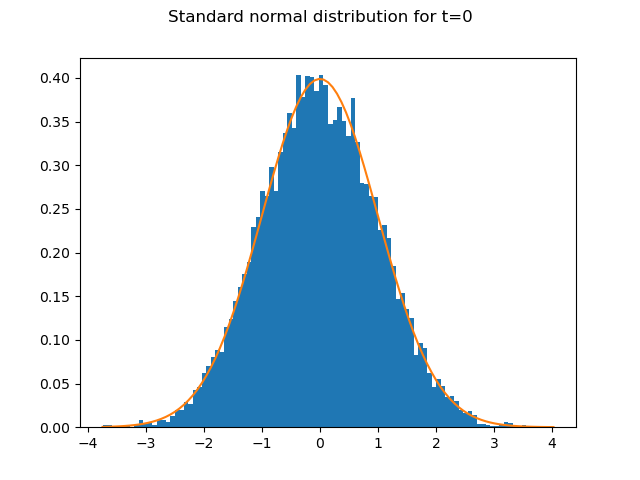
10,000 random numbers drawn from the standard normal distribution are generated for each time step. The graph shows how well the 10,000 random numbers for t=0 fit the PDF of the standard normal distribution.

import modelx as mx
import pandas as pd
import matplotlib.pyplot as plt
from scipy.stats import norm, lognorm
import numpy as np

model = mx.read_model("CashValue_ME_EX1")
rand_nums = model.Projection.std_norm_rand()
pv_avs = model.Projection.pv_claims_from_av('MATURITY')
num_bins = 100
S0 = 45000000
sigma = 0.03
T = 10

fig, ax = plt.subplots()
n, bins, patches = ax.hist(rand_nums[:, 0], bins=num_bins, density=True)
ax.plot(bins, norm.pdf(bins), '-')
fig.suptitle('Standard normal distribution for t=0')

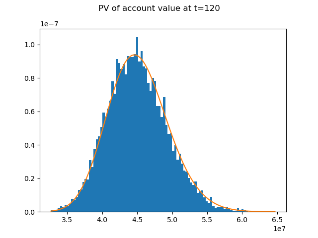
The distibution of the account value at t=120 follows a log normal distribution. In the expression below, \(S_{T}\) and \(S_{0}\) denote the account value at t=T=120 and t=0 respectively.

\[\ln\frac{S_{T}}{S_{0}}\sim\phi\left[\left(r-\frac{\sigma^{2}}{2}\right)T, \sigma\sqrt{T}\right]\]

The graph shows how well the distribution of \(e^{-rT}S_{T}\), the present values of the account value at t=0, fits the PDF of a log normal ditribution.

Reference: Options, Futures, and Other Derivatives by John C.Hull

See also

• 1. Simple Stochastic Example notebook in the savings library

fig, ax = plt.subplots()
n, bins, patches = ax.hist(pv_avs, bins=num_bins, density=True)
ax.plot(bins, lognorm.pdf(bins, sigma * T**0.5, scale=S0), '-')
fig.suptitle('PV of account value at t=120')