Note
Go to the end to download the full example code.
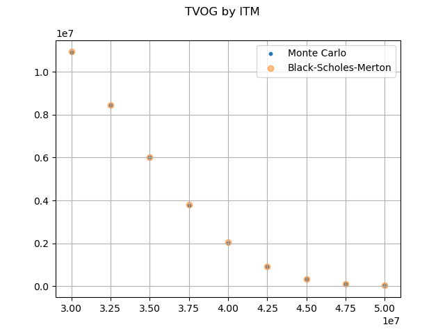
Monte Carlo vs Black-Scholes-Merton#
Time values of options and guarantees for various in-the-moneyness are calculated using Monte Carlo simulations and the Black-Scholes-Merton pricing formula for European put options.
The Black-Scholes-Merton pricing formula for European put options can be expressed as below, where \(X\) and \(S_{0}\) correspond to the sum assured and the initial account value in this example.
The graph below shows the results obtained from the Monte Carlo simulations with 10,000 risk neutral scenarios, and from the Black-Scholes-Merton formula.
Reference: Options, Futures, and Other Derivatives by John C.Hull
See also
1. Simple Stochastic Example notebook in the
savingslibrary
import modelx as mx
import pandas as pd
import matplotlib.pyplot as plt
from scipy.stats import norm, lognorm
import numpy as np

model = mx.read_model("CashValue_ME_EX1")
proj = model.Projection
proj.model_point_table = proj.model_point_moneyness
monte_carlo = pd.Series(proj.pv_claims_over_av('MATURITY'), index=proj.model_point().index)
monte_carlo = list(np.average(monte_carlo[i]) for i in range(1, 10))
S0 = proj.model_point_table['premium_pp'] * proj.model_point_table['policy_count']


fig, ax = plt.subplots()
ax.scatter(S0, monte_carlo, s= 10, alpha=1, label='Monte Carlo')
ax.scatter(S0, proj.formula_option_put(120), alpha=0.5, label='Black-Scholes-Merton')
ax.legend()
ax.grid(True)
fig.suptitle('TVOG by ITM')
Total running time of the script: (0 minutes 2.451 seconds)