Note
Go to the end to download the full example code.
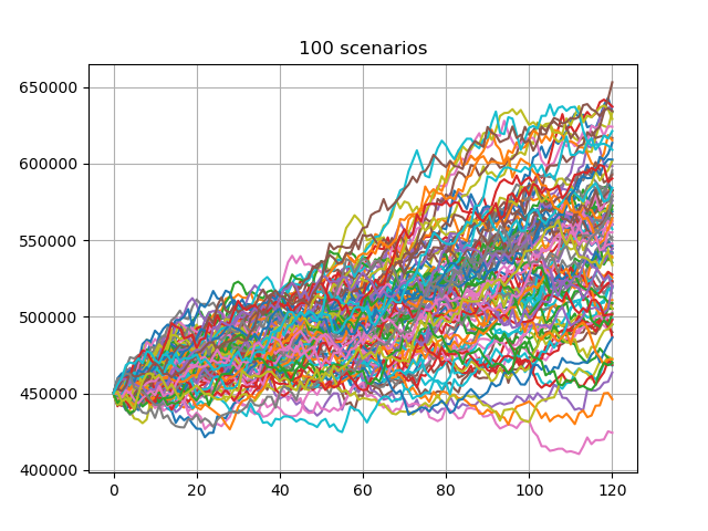
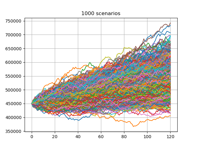
Account value paths#
Account value paths generated by the Monte Carlo simulation. The first 100 and 1000 paths out of 10000 are plotted.
The investment return on account value is modeled to follow the following geometric Brownian motion
\[\frac{\Delta{S}}{S}=r\Delta{t}+\sigma\epsilon\sqrt{\Delta{t}}\]
where \(\Delta{S}\) is the change in the account value \(S\), in a small interval of time, \(\Delta{t}\), \(r\) is the constant risk free rate, \(\sigma\) is the volatility of the account value and \(\epsilon\) is a random number drawn from the standard normal distribution.
See also
1. Simple Stochastic Example notebook in the
savingslibrary
import modelx as mx
import pandas as pd

model = mx.read_model("CashValue_ME_EX1")
proj = model.Projection
av = proj.av_pp_at

avs = list(av(t, 'BEF_FEE') for t in range(proj.max_proj_len()))
df = pd.DataFrame(avs)[1]

for scen_size in [100, 1000]:
    df[range(1, scen_size + 1)].plot.line(
        legend=False, grid=True, title="%s scenarios" % scen_size)
Total running time of the script: (0 minutes 2.112 seconds)