Note
Go to the end to download the full example code.
Discount factor convergence#
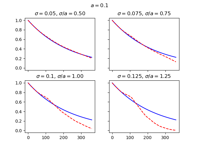
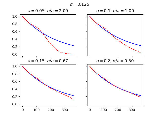
The convergence of the stochastic discount factors generated by the Hull-White model.
The charts below examine the convergence of the discount factors for various combinations of \(\sigma\) and \(a\), first by changing \(\sigma\) and secondly by changing \(a\). As Balaraman’s study shows, the convergence gets worse as \(\sigma/a\) gets larger than 1, and gets better as \(\sigma/a\) gets smaller than 1.
See also
Overview of BasicHullWhite notebook in the
economiclibrary
import modelx as mx
import matplotlib.pyplot as plt

HW = mx.read_model("BasicHullWhite").HullWhite

fig, axs = plt.subplots(2, 2, sharex=True, sharey=True)
fig.suptitle(r"$a=$" + str(HW.a))
for sigma, (h, v) in zip([0.05, 0.075, 0.1, 0.125], [(0, 0), (0, 1), (1, 0), (1, 1)]):
    HW.sigma = sigma
    axs[h, v].set_title(r"$\sigma=$" + str(sigma) +  r", $\sigma/a=$" + "%.2f" % (sigma/HW.a))
    axs[h, v].plot(range(HW.step_size+1), [HW.mkt_zcb(i) for i in range(HW.step_size+1)], "b-")
    axs[h, v].plot(range(HW.step_size+1), HW.mean_disc_factor(), "r--")

fig, axs = plt.subplots(2, 2, sharex=True, sharey=True)
fig.suptitle(r"$\sigma=$" + str(HW.sigma))
HW.sigma = 0.1
for a, (h, v) in zip([0.05, 0.1, 0.15, 0.2], [(0, 0), (0, 1), (1, 0), (1, 1)]):
    HW.a = a
    axs[h, v].set_title(r"$a=$" + str(a) +  r", $\sigma/a=$" + "%.2f" % (HW.sigma/HW.a))
    axs[h, v].plot(range(HW.step_size+1), [HW.mkt_zcb(i) for i in range(HW.step_size+1)], "b-")
    axs[h, v].plot(range(HW.step_size+1), HW.mean_disc_factor(), "r--")
Total running time of the script: (0 minutes 0.790 seconds)