Quick Start#
Getting lifelib#
If you are on Windows, simply download lifelib with WinPython from here. Unzip the file. No installation is required. The file contains a custom Python distribution based on WinPython distribution, which includes preinstalled lifelib, modelx, spyder-modelx and all other relevant packages.
If you are on Linux or Mac, follow the manual installation instruction below. If you do not wish to use the WinPython-based distribution, and want to use lifelib on your Anaconda environment, follow the instruction.
Using lifelib with Spyder#
Spyder is a popular scientific Python IDE, and it’s bundled in with WinPython by default. Spyder plugin for modelx adds widgets to Spyder, which enable you to graphically interface with lifelib models and to develop, run and analyze the models more efficiently. Below are the widgets installed by the plugin.
Starting Spyder#
To launch Spyder, go to the unzipped folder, and run Spyder.exe by double-clicking it. If you’re using Anaconda, you should be able to launch Spyder from Windows menu.
Copying a Library#
lifelib is essentially a collection of folders called libraries, which contain models and some other files. You can create your copy of a library, either from IPython console or from command prompts.
Creating a library copy from IPython
You can create a copy of a lifelib library from Spyder’s IPython console using
lifelib.create function:
>>> import lifelib

>>> lifelib.create("basiclife", "mylife")
The first parameter is the name of the lifelib library to copy.
The second parameter is the folder path to create.
If only a folder name is given, the folder is created under the current
folder.
The Files widget in Spyder shows where the current folder is.
Alternatively, the current folder can be reported by os.getcwd function:
>>> import os

>>> os.getcwd()
If the second argument is omitted, the first parameter, which is the library name is used.
Creating a library from command prompt
Alternatively, you can copy a library
by a command lifelib-create from the command prompt
named “WinPython Command Prompt.exe” included in the unzipped folder.
For example, to create a project folder named
mylife under the path C:\Users\fumito by copying lifelib’s default
library basiclife,
Go to the unzipped folder and start WinPython Command Prompt.exe. Type the following command on the command prompt:
> lifelib-create --template basiclife C:\Users\fumito\mylife
Alternatively, since basiclife is the default library,
you can get away with –template option like this:
> lifelib-create C:\Users\fumito\mylife
Reading a Model#
The created folder contains folders whose names start with model_.
Those are model folders. By reading a model folder into an IPython session,
a live Model object is created.
For example,
the BasicTerm_S
model in basiclife is saved as a folder named BasicTerm_S.
To read the model,
start an MxConsole session by right-clicking on Console 1/A tab
and select New MxConsole.
Next, right-click on the blank space in MxExplorer
to bring up a context menu.
Select Read Model item from the menu.
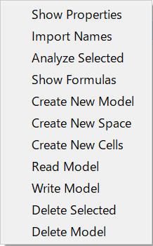
MxExplorer’s context menu#
Click the folder icon next to the text box at the top, select the BasicTerm_S folder in the created folder then click OK. After model is read successfully, the components of the model appear as a tree in the MxExplorer. The top item in the tree is Projection, and it represents the Projection Space in the model. The space object contains child objects. Double-click on Projection to expand it and show Projection’s child objects.
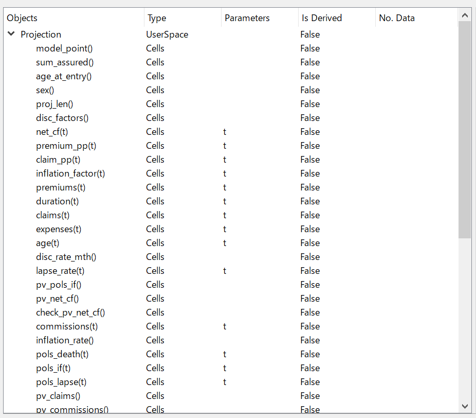
MxExplorer showing Projection and its child objects#
Importing Names#
In the MxConsole, the model is defined as a variable named BasicTerm_S as you see in the Variable Explorer widget, so typing BasicTerm_S in the MxConsole returns the model:
>>> BasicTerm_S
<Model BasicTerm_S>
Projection, and its child objects are not defined in the MxConsole, and they can be retrieved as the attributes of their parents:
>>> BasicTerm_S.Projection
<UserSpace BasicTerm_S.Projection>

>>> BasicTerm_S.Projection.model_point
<Cells BasicTerm_S.Projection.model_point()>
Auto-completion works in the MxConsole, so type the first couple of characters then hit Tab to complete the remainder. To access these objects more quickly, you can define variables that refer to the objects. There is a way to define variables for a Space and all of its child objects at once. In MxExplorer, select Projection in the object tree, and right-click to show the context menu, and select Import Names from the menu.
The dialog box below shows up. Click OK.
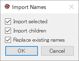
Import Names dialog box#
Now, you see the Projection space and all the child object in the space are defined as global variables in the MxConsole as you see in the Variable Explorer.
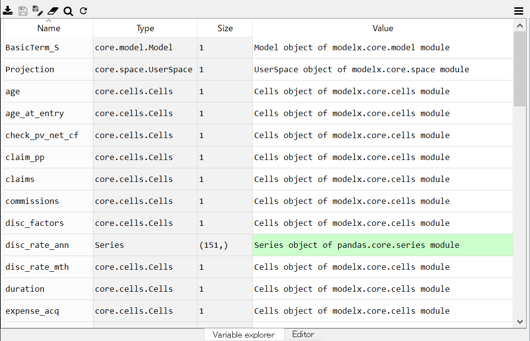
Variable Explorer showing defined global variables#
Calculating Values#
Most of the child objects are Cells object. A Cells acts like a function, but instead of always calculating the value for the same arguments, it calculates the value for the same arguments only once, and keep the returned value until the Cells needs to be refreshed. The calculation logic of a Cells is defined by a Python function as a Formula object. To calculate the value of a Cells for certain arguments, simply call the Cells with the arguments:
>>> claims(0)
34.18079328868595
In the BasicTerm_S model, the result_cf Cells returns the projected
cashflow result of a selected model point
as a DataFrame object. It does not take any arguments:
>>> result_cf()
      Premiums     Claims    Expenses  Commissions  Net Cashflow
0    94.840000  34.180793  300.000000    94.840000   -334.180793
1    94.005734  33.880120    4.956017    94.005734    -38.836137
2    93.178806  33.582091    4.912421    93.178806    -38.494512
3    92.359153  33.286684    4.869209    92.359153    -38.155893
4    91.546710  32.993876    4.826377    91.546710    -37.820252
..         ...        ...         ...          ...           ...
116  62.432465  63.534771    3.599824     0.000000     -4.702130
117  62.317757  63.418038    3.593210     0.000000     -4.693491
118  62.203260  63.301519    3.586608     0.000000     -4.684868
119  62.088973  63.185215    3.580019     0.000000     -4.676260
120   0.000000   0.000000    0.000000     0.000000      0.000000

[121 rows x 5 columns]
The result_pv Cells returns a DataFrame that shows
the present values of the cashflows
and their percentages to the present value of premiums:
>>> result_pv()
              Premiums       Claims    Expenses  Commissions  Net Cashflow
PV         8251.931435  5501.074678  748.303591  1084.601434    917.951731
% Premium     1.000000     0.666641    0.090682     0.131436      0.111241
Viewing Values#
The MxDataViewer widget is useful for viewing values contained in Cells and Reference objects, especially when they hold vector or tabular data, such as pandas Series, DataFrames and numpy arrays.
For example, to view the values of result_cf,
double-click on result_cf in MxExplorer to show
BasicTerm_S.Projection.result_cf at the top of MxDataViewer,
then click Update.
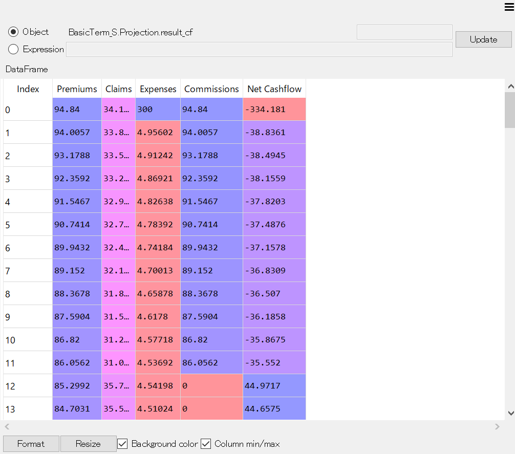
MxDataViewer showing result_cf#
Tracing Calculations#
The MxAnalyzer widget is useful for tracing values and formulas used for calculating a value of a specific Cells.
For example, to trace the calculations of result_cf,
select result_cf in MxExplorer and right-click to bring up
the context menu, then from the menu select Analyzer Selected.
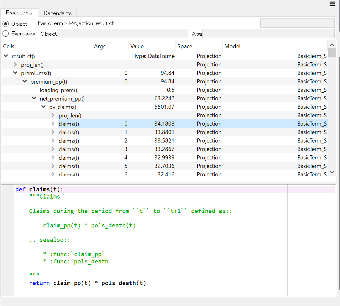
MxAnalyzer showing the dependency tree of result_cf#
Running Notebooks#
Running Notebooks online#
Jupyter Notebook enables you to run Python code in your browser. lifelib comes with some Jupyter notebooks, and the quickest way to try lifelib is to run the notebooks online. Go to Notebooks page and click one of the banner links. The link will take you to a web page where the selected notebook starts loading. Once the notebook loads, select Cell menu, and then select Run All to run & build models and get results and draw graphs.
Running Notebooks locally#
Jupyter notebooks on Notebooks page are also included in lifelib
projects, and can be executed on your local computer by running
Jupyter Notebook locally.
For example, if you create a project folder named myifrs17sim from
the project template ifrs17sim,
you can go to the folder by cd command and launch Jupyter Notebook:
> cd myifrs17sim

> jupyter notebook
The command above opens a new tab in your web browser, and Jupyter Notebook session starts in the tab.
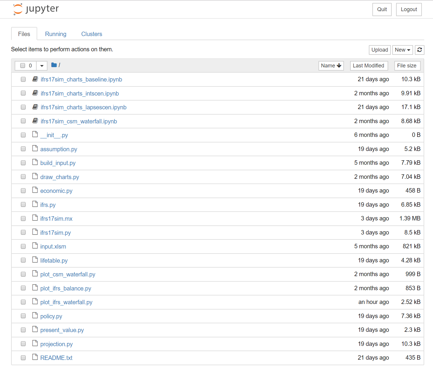
files with ipynb extension are Jupyter notebooks. By double-clicking one,
it opens in another tab, and you’ll see the same page as you see it online.