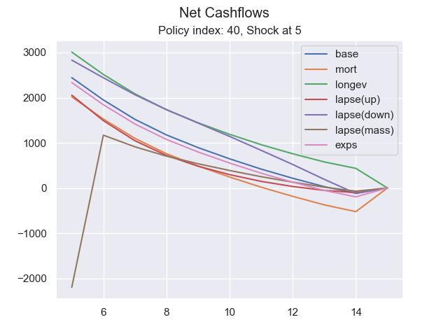
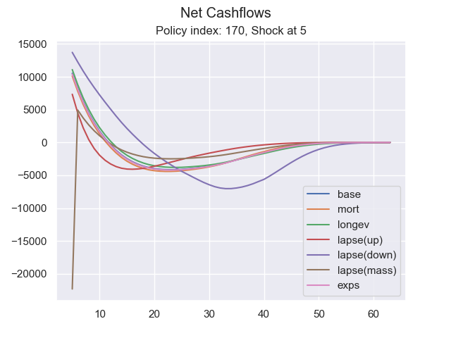
TradLife_A_EX1: SCR shock cashflows

Net liability cashflows under the prescribed Solvency II life shock scenarios for selected policies, projected by the annuallife TradLife_A_EX1 model.

For each policy the inner projection InnerProj[t0, risk, shock] is re-run from the valuation time t0 under every life stress, and the per-period net cashflow net_cf is charted from t0 to the end of the projection. The mass-lapse line drops sharply at t0 because a fraction of the policies surrenders instantly under that shock.

See also

• The annuallife library

• 
• 

import modelx as mx
import pandas as pd
import matplotlib.pyplot as plt
import seaborn as sns
sns.set_theme(style="darkgrid")

model = mx.read_model("TradLife_A_EX1")
LifeRiskID = model.Enums.LifeRiskID
LapseShockID = model.Enums.LapseShockID

# (label, risk, shock) for each prescribed life stress
scenarios = [
    ('base', LifeRiskID.BASE, 0),
    ('mort', LifeRiskID.MORT, 0),
    ('longev', LifeRiskID.LONGV, 0),
    ('lapse(up)', LifeRiskID.LAPSE, LapseShockID.UP),
    ('lapse(down)', LifeRiskID.LAPSE, LapseShockID.DOWN),
    ('lapse(mass)', LifeRiskID.LAPSE, LapseShockID.MASS),
    ('exps', LifeRiskID.EXPS, 0),
]


def draw(idx, t0):

    fig, ax = plt.subplots()
    fig.suptitle('Net Cashflows')

    title = 'Policy index: ' + str(idx) + ', Shock at ' + str(t0)

    proj = model.Projection[idx]
    last_t = proj.proj_len()

    data = {}
    for label, risk, shock in scenarios:
        inner = proj.InnerProj[t0, risk, shock]
        data[label] = [inner.net_cf(t) for t in range(t0, last_t + 1)]

    return pd.DataFrame(
        data, index=range(t0, last_t + 1)).plot(
        ax=ax, kind='line', title=title)


# idx 40 / 170 correspond to PolicyID 41 / 171 in simplelife (0-based).
for idx, t0 in [(40, 5), (170, 5)]:
    draw(idx, t0)