The BasicTerm_S Model

Overview

The BasicTerm_S model is the most basic cashflow model in lifelib.

The model is a monthly step, new business model and projects insurance cashflows of a sample model point. The modeled product is a level-premium plain term product with no surrender value. The projected cashflows are premiums, claims, expenses and commissions. The assumptions used are mortality rates, lapse rates, discount rates, expense, inflation and commission rates. The present values of the cashflows are also calculated. The premium amount for each individual model point is calculated as the net premium with loadings, where the net premium is calculated from the present value of the claims.

Basic Usage

Reading the model

Create your copy of the basiclife library by following the steps on the Quick Start page. The model is saved as the folder named BasicTerm_S in the copied folder.

To read the model from Spyder, right-click on the empty space in MxExplorer, and select Read Model. Click the folder icon on the dialog box and select the BasicTerm_S folder.

Getting the results

By default, the model has Cells for outputting projection results as listed in the Results section. result_cf() outputs cashflows of the selected model point, and result_pv() outputs the present values of the cashflows. Both Cells outputs the results as pandas DataFrame.

See the Quick Start page for how to get the results in an MxConsole and view the results in MxDataViewer.

Changing the model point

The model point to be selected is determined by point_id in Projection. It is 1 by default. model_point_table contains all the 10,000 sample model points as a pandas DataFrame. To change the model point to another one, set the other model point’s ID to point_id. Setting the new point_id clears all the values of Cells that are specific to the previous model point.

Getting multiple results

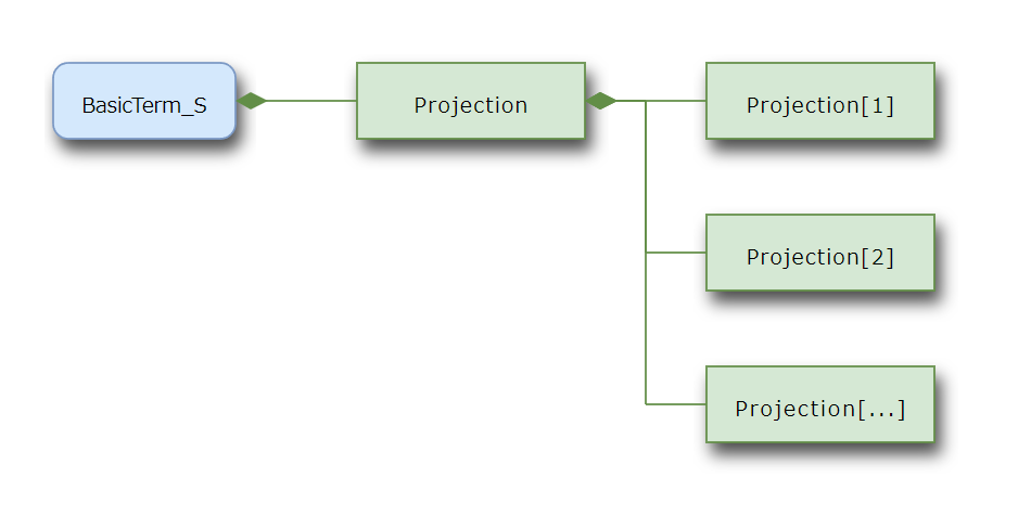
The Projection space is parameterized with point_id, i.e. the Projection space can have dynamic child spaces, such as Projection[1], Projection[2], Projection[3] …, each of which represents the Projection for each of the model points.

Note

Getting results for too many dynamic child spaces takes a considerable amount of time. The default BasicTerm_S model would take more than a minute for 1000 model points on an ordinary spec PC. To calculate for many model points, consider using the BasicTerm_M model.

Model Specifications

The BasicTerm_S model has only one UserSpace, named Projection, and all the Cells and References are defined in the space.

The Projection Space

The main Space in the BasicTerm_S model.

Projection is the only Space defined in the BasicTerm_S model, and it contains all the logic and data used in the model.

Parameters and References

(In all the sample code below, the global variable Projection refers to the Projection Space.)

point_id

The ID of the selected model point. point_id is defined as a Reference, and its value is used for determining the selected model point. By default, 1 is assigned. To select another model point, assign its model point ID to it:

>>> Projection.point_id = 2

point_id is also defined as the parameter of the Projection Space, which makes it possible to create dynamic child space for multiple model points:

>>> Projection.parameters
('point_id',)

>>> Projection[1]
<ItemSpace BasicTerm_S.Projection[1]>

>>> Projection[2]
<ItemSpace BasicTerm_S.Projection[2]>

See also

• model_point_table

• model_point()

model_point_table

All model point data as a DataFrame. The sample model point data was generated by generate_model_points.ipynb included in the library. The DataFrame has an index named point_id, and model_point() returns a record as a Series whose index value matches point_id. The DataFrame has columns labeled age_at_entry, sex, policy_term, policy_count and sum_assured. Cells defined in Projection with the same names as these columns return the corresponding column’s values for the selected model point. (policy_count is not used by default.)

>>> Projection.model_poit_table
           age_at_entry sex  policy_term  policy_count  sum_assured
point_id
1                    47   M           10             1       622000
2                    29   M           20             1       752000
3                    51   F           10             1       799000
4                    32   F           20             1       422000
5                    28   M           15             1       605000
                ...  ..          ...           ...          ...
9996                 47   M           20             1       827000
9997                 30   M           15             1       826000
9998                 45   F           20             1       783000
9999                 39   M           20             1       302000
10000                22   F           15             1       576000

[10000 rows x 5 columns]

The DataFrame is saved in the Excel file model_point_table.xlsx placed in the model folder. model_point_table is created by Projection’s new_pandas method, so that the DataFrame is saved in the separate file. The DataFrame has the injected attribute of _mx_dataclident:

>>> Projection.model_point_table._mx_dataclient
<PandasData path='model_point_table.xlsx' filetype='excel'>

See also

• point_id

• model_point()

• age_at_entry()

• sex()

• policy_term()

• sum_assured()

disc_rate_ann

Annual discount rates by duration as a pandas Series.

>>> Projection.disc_rate_ann
year
0      0.00000
1      0.00555
2      0.00684
3      0.00788
4      0.00866

146    0.03025
147    0.03033
148    0.03041
149    0.03049
150    0.03056
Name: disc_rate_ann, Length: 151, dtype: float64

The Series is saved in the Excel file disc_rate_ann.xlsx placed in the model folder. disc_rate_ann is created by Projection’s new_pandas method, so that the Series is saved in the separate file. The Series has the injected attribute of _mx_dataclident:

>>> Projection.disc_rate_ann._mx_dataclient
<PandasData path='disc_rate_ann.xlsx' filetype='excel'>

See also

• disc_rate_mth()

• disc_factors()

mort_table

Mortality table by age and duration as a DataFrame. See basic_term_sample.xlsx included in this library for how the sample mortality rates are created.

>>> Projection.mort_table
            0         1         2         3         4         5
Age
18   0.000231  0.000254  0.000280  0.000308  0.000338  0.000372
19   0.000235  0.000259  0.000285  0.000313  0.000345  0.000379
20   0.000240  0.000264  0.000290  0.000319  0.000351  0.000386
21   0.000245  0.000269  0.000296  0.000326  0.000359  0.000394
22   0.000250  0.000275  0.000303  0.000333  0.000367  0.000403
..        ...       ...       ...       ...       ...       ...
116  1.000000  1.000000  1.000000  1.000000  1.000000  1.000000
117  1.000000  1.000000  1.000000  1.000000  1.000000  1.000000
118  1.000000  1.000000  1.000000  1.000000  1.000000  1.000000
119  1.000000  1.000000  1.000000  1.000000  1.000000  1.000000
120  1.000000  1.000000  1.000000  1.000000  1.000000  1.000000

[103 rows x 6 columns]

The DataFrame is saved in the Excel file mort_table.xlsx placed in the model folder. mort_table is created by Projection’s new_pandas method, so that the DataFrame is saved in the separate file. The DataFrame has the injected attribute of _mx_dataclident:

>>> Projection.mort_table._mx_dataclient
<PandasData path='mort_table.xlsx' filetype='excel'>

See also

• mort_rate()

• mort_rate_mth()

np

The numpy module.

pd

The pandas module.

Projection parameters

This is a new business model and all model points are issued at time 0. The time step of the model is monthly. Cashflows and other time-dependent variables are indexed with t.

Cashflows and other flows that accumulate throughout a period indexed with t denote the sums of the flows from t til t+1. Balance items indexed with t denote the amount at t.

proj_len()

Projection length in months

Model point data

The model point data is stored in an Excel file named model_point_table.xlsx under the model folder.

model_point()	The selected model point as a Series
sex()	The sex of the selected model point
sum_assured()	The sum assured of the selected model point
policy_term()	The policy term of the selected model point.
age(t)	The attained age at time t.
age_at_entry()	The age at entry of the selected model point
duration(t)	Duration in force in years

Assumptions

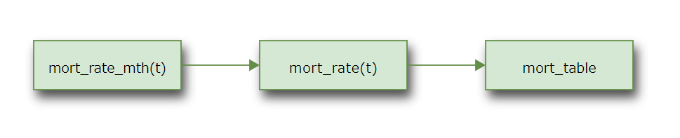
The mortality table is stored in an Excel file named mort_table.xlsx under the model folder, and is read into mort_table as a DataFrame. mort_rate() looks up mort_table and picks up the annual mortality rate to be applied for the selected model point at time t. mort_rate_mth() converts mort_rate() to the monthly mortality rate to be applied during the month starting at time t.

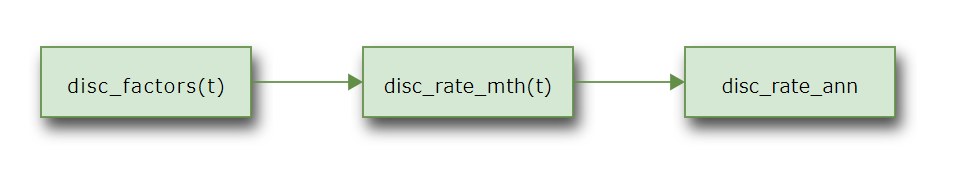
The discount rate data is stored in an Excel file named disc_rate_ann.xlsx under the model folder, and is read into disc_rate_ann as a Series.

The lapse by duration is defined by a formula in lapse_rate(). expense_acq() holds the acquisition expense per policy at t=0. expense_maint() holds the maintenance expense per policy per annum. The maintenance expense inflates at a constant rate of inflation given as inflation_rate().

mort_rate(t)	Mortality rate to be applied at time t
mort_rate_mth(t)	Monthly mortality rate to be applied at time t
disc_factors()	Discount factors.
disc_rate_mth()	Monthly discount rate
lapse_rate(t)	Lapse rate
expense_acq()	Acquisition expense per policy
expense_maint()	Annual maintenance expense per policy
inflation_factor(t)	The inflation factor at time t
inflation_rate()	Inflation rate

Policy values

By default, the amount of death benefit for each policy (claim_pp()) is set equal to sum_assured.

The payment method is monthly whole term payment for all model points. The monthly premium per policy (premium_pp()) is calculated for each policy as (1 + loading_prem()) times net_premium_pp(). The net premium is calculated so that the present value of the net premiums equates to the present values of claims.

This product is assumed to have no surrender value.

claim_pp(t)	Claim per policy
net_premium_pp()	Net premium per policy
loading_prem()	Loading per premium
premium_pp()	Monthly premium per policy

Policy decrement

The initial number of policies is set to 1 per model point by default, and decreases through out the policy term by lapse and death. At the end of the policy term the remaining number of policies mature.

pols_death(t)	Number of death occurring at time t
pols_if(t)	Number of policies in-force
pols_if_init()	Initial Number of Policies In-force
pols_lapse(t)	Number of lapse occurring at time t
pols_maturity(t)	Number of maturing policies

Cashflows

An acquisition expense at t=0 and maintenance expenses thereafter comprise expense cashflows.

Commissions are assumed to be paid out during the first year and the commission amount is assumed to be 100% premium during the first year and 0 afterwards.

claims(t)	Claims
commissions(t)	Commissions
premiums(t)	Premium income
expenses(t)	Acquisition and maintenance expenses
net_cf(t)	Net cashflow

Present values

The Cells whose names start with pv_ are for calculating the present values of the cashflows indicated by the rest of their names. pols_if() is not a cashflow, but used as an annuity factor in calculating net_premium_pp().

pv_claims()	Present value of claims
pv_commissions()	Present value of commissions
pv_expenses()	Present value of expenses
pv_net_cf()	Present value of net cashflows.
pv_pols_if()	Present value of policies in-force
pv_premiums()	Present value of premiums
check_pv_net_cf()	Check present value summation

Results

result_cf() outputs the cashflows of the selected model point as a DataFrame:

>>> result_cf()
      Premiums     Claims  ...  Policies Death  Policies Exits
0    94.840000  34.180793  ...        0.000055        0.008742
1    94.005734  33.880120  ...        0.000054        0.008665
2    93.178806  33.582091  ...        0.000054        0.008588
3    92.359153  33.286684  ...        0.000054        0.008513
4    91.546710  32.993876  ...        0.000053        0.008438
..         ...        ...  ...             ...             ...
116  62.432465  63.534771  ...        0.000102        0.001107
117  62.317757  63.418038  ...        0.000102        0.001105
118  62.203260  63.301519  ...        0.000102        0.001103
119  62.088973  63.185215  ...        0.000102        0.001101
120   0.000000   0.000000  ...        0.000000        0.000000

[121 rows x 8 columns]

result_pv() outputs the present values of the cashflows and also their percentages against the present value of premiums as a DataFrame:

>>> result_pv()
              Premiums       Claims    Expenses  Commissions  Net Cashflow
PV         8251.931435  5501.074678  748.303591  1084.601434    917.951731
% Premium     1.000000     0.666641    0.090682     0.131436      0.111241

result_cf()	Result table of cashflows
result_pv()	Result table of present value of cashflows